New and improved GAMS links for Pyomo and JuMP

We have developed a new interface between JuMP and GAMS, and improved the existing interface between Pyomo and GAMS.

Background

Using GDX is currently the most efficient way to exchange data (like variable and equations solution records) with GAMS. Many (mostly academic) GAMS users also use other modeling tools, such as JuMP (Julia) or Pyomo (Python). Both of these have gained quite some traction in recent years, and interfacing them with GAMS in an efficient way is something that has been requested by some people. Our developers have therefore spent some time utilizing GDX to interface GAMS with Pyomo and JuMP as efficiently as possible.

JuMP

For a relatively new programming language, Julia has gained a lot of attention, because of its straightforward syntax that makes algebraic expressions easy, and for its execution speed that approaches that of compiled languages. JuMP is a Julia package for mathematical modeling and supports a range of different solvers. However, many users want to use solvers that are not supported by JuMP, but come with GAMS. Currently these are: AlphaECP, Antigone, Conopt, DICOPT, GLOMIQO, LGO, LINDO, LINDOGLOBAL, Localsolver, MINOS, MSNLP, ODHCPLEX, PATHNLP, SBB, SHOT, SNOPT, SoPLEX, XA and our own development BDMLP. We have developed a new interface (https://github.com/GAMS-dev/gams.jl ) that allows using GAMS as a JuMP solver:

using GAMS
using JuMP

model = Model(GAMS.Optimizer)

I = 1:2
J = 1:3

a = [350, 600]
b = [325, 300, 275]
d = [2.5 1.7 1.8; 2.5 1.8 1.4]

@variable(model, x[I,J] >= 0)

@objective(model, Min, 0.09 * sum(d[i,j] * x[i,j] for i in I, j in J))

@constraint(model, [i in I], sum(x[i,j] for j in J) <= a[i])
@constraint(model, [j in J], sum(x[i,j] for i in I) >= b[j])

JuMP.optimize!(model)

println("Optimal Solution: ", JuMP.objective_value(model))

The new interface supports the following JuMP features:

• linear, quadratic and nonlinear (convex and non-convex) objective and constraints
• continuous, binary, integer, semi-continuous and semi-integer variables
• SOS1 and SOS2 sets

Pyomo

Pyomo allows formulating, solving, and analyzing optimization models in Python. Pyomo has already had a GAMS interface . We have recently contributed to the Pyomo project to improve the performance of the interface by using GDX.

Use GAMS as Pyomo solver:

from pyomo.environ import *
opt = SolverFactory('gams')

model = ConcreteModel()

model.i = RangeSet(0,1)
model.j = RangeSet(0,2)

a = [350, 600]
b = [325, 300, 275]
d = [[2.5, 1.7, 1.8], [2.5, 1.8, 1.4]]

model.x = Var(model.i, model.j, domain=NonNegativeReals)

model.obj = Objective(expr=0.09 * sum(d[i][j] * model.x[i,j] for i in model.i for j in model.j))

def c1_rule(model, i):
    return sum(model.x[i,j] for j in model.j) <= a[i]
model.c1 = Constraint(model.i, rule=c1_rule)

def c2_rule(model, j):
    return sum(model.x[i,j] for i in model.i) >= b[j]
model.c2 = Constraint(model.j, rule=c2_rule)

results = opt.solve(model)

print('Optimal Solution: ', value(model.obj))

As an added bonus you can use our GAMS convert tool to convert GAMS instances (.gms) to Pyomo models (.py)

How does this work?

We followed the same principles in both interfaces:

• When solving a model with the GAMS solver (or MathOptInterface Optimizer), a GMS text file with a scalar model (similar to https://www.gams.com/latest/docs/S_CONVERT.html#INDEX_CONVERT_22_scalar_21_model ) is created and executed by a GAMS shell command.
• The generated model instance is passed to a GAMS solver link and the actual solver starts to work on a solution.
• When the solver terminates, the solution point and status is exported to a GDX file, which is read using the gdxcc Python module or direct C calls to the GAMS GDX library libgdxdclib64.so (in case of Julia).

The upshot

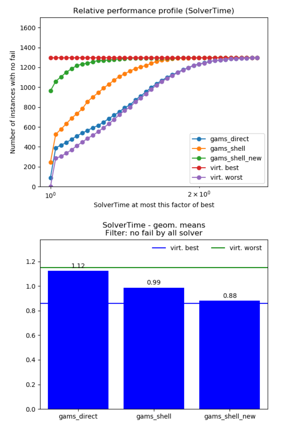
With the newly developed / improved link we have an efficient interface. In the case of Pyomo, we can demonstrate significant performance improvements.