Introducing: GAMS Transfer

The object oriented APIs that come with every GAMS installation are a great way to seamlessly integrate GAMS modeling into existing applications and IT environments. You can choose from .NET, C++, Java, Python, and Matlab. The last two from this list are particularly popular with those who need to analyse data in an exploratory and interactive fashion.

In the Python community, Pandas is a commonly used package that allows convenient storing and manipulation of data, with advanced operations for indexing and slicing, reshaping, merging and visualization of data.

In Matlab, the builtin matrix, table and struct formats are the commonly used data structures to manipulate data.

For both Python and Matlab, the existing GAMS APIs are very powerful and feature complete, but working interactively with GAMS data can be tedious. We have therefore started a new project called GAMS Transfer (part of GAMS 37), with the aim to create an API dedicated to data exchange between GAMS and other languages, starting with Python and Matlab.

In the GAMS Transfer project we focus on several key points:

• Speed: Performance is critical for large datasets
• Convenience: The API must be intuitive to use and use environment specific data formats
• Consistency: Use of analogous syntax across different environments

Our team first presented GAMS Transfer to the public at the 2021 Informs Annual Meeting. .

A key element of GAMS Transfer is the concept of a container, which is the repository that holds all data. Data within this container is linked together, which enables data operations like implicit set growth, domain checking, data format transformations (to dense/sparse matrix formats), etc. Those concepts are explained in more detail in the documentation for Python and for Matlab .

Below we will use a simple example to demonstrate how the GAMS Transfer API integrates seamlessly with Python. We will

• write some data to a GDX file with GAMS Transfer,
• start a GAMS job that will use the created GDX file (using the traditional GAMS Python API),
• and then read the results back into a Python dataframe with GAMS Transfer and plot the data on a map.

The point here is not to explore all aspects of GAMS Transfer, but instead highlight how easy it is to get started.

An Example Using the TRANSPORT Model

This simple example is based on the TRANSPORT model from our model library. For the example, we modify the model to load the Set and Parameter data from the GDX file we will produce with GAMS Transfer:

GAMS Model

 1
 2
 3
 4
 5
 6
 7
 8
 9
10
11
12
13
14
15
16
17
18
19
20
21
22
23
24
25
26
27
28
29
30
31
32
33
34
35
36
37
38
39
40
41
42
43
44
45
46
47
48

$eolCom #
$gdxIn input_data.gdx  # Open the GAMS Transfer GDX file for input

Set
   i 'canning plants' 
   j 'markets';
$load i j   # Load set members from GDX 

Parameter
   a(i) 'capacity of plant i in cases'
   b(j) 'demand at market j in cases';
$load a b   # Load Parameter data from GDX

Table d(i,j) 'distance in thousands of miles';
$load d     # Load distances from GDX

Scalar f 'freight in dollars per case per thousand miles';
$load f    # Load cost scalar 

Parameter c(i,j) 'transport cost in thousands of dollars per case';
c(i,j) = f*d(i,j)/1000;  # This calculation uses the loaded GDX data!

$gdxin      # close the gdx file


# The rest of the model does not need to be modified

Variable
   x(i,j) 'shipment quantities in cases'
   z      'total transportation costs in thousands of dollars';

Positive Variable x;


Equation
   cost      'define objective function'
   supply(i) 'observe supply limit at plant i'
   demand(j) 'satisfy demand at market j';

cost..      z =e= sum((i,j), c(i,j)*x(i,j));

supply(i).. sum(j, x(i,j)) =l= a(i);

demand(j).. sum(i, x(i,j)) =g= b(j);

Model transport / all /;

solve transport using lp minimizing z;

Now let’s get to using GAMS Transfer with Python. First, we need to import a few packages. Apart from GAMS Transfer itself we will use Pandas dataframes in the example. Also, we have a couple of helper functions (get_locations, calculate_distances) that will calculate distances between cities. The listing of geo.py will be included at the bottom of this post.

import gamstransfer as gt
import pandas as pd
import os

from geo import get_locations, calculate_distances

working_dir = os.getcwd()
model_name  = "trnsport_gamsxfer_gdx"  # The name of the GAMS model file

Geographical locations are retrieved for a list of production plant cities, and for a list of market cities:

plants  = ['seattle','san-diego']
markets = ['new-york','chicago','topeka','denver']

plant_locations  = get_locations(plants)
market_locations = get_locations(markets)

The distances between plants and markets are calculated and used to populate a Pandas dataframe

distances = pd.DataFrame(data=calculate_distances(plant_locations,market_locations), columns = ['from', 'to', 'distance (1000 mi)'])
distances

We also have to add production capacity (cap) of each plant, and demand (dem) for each market:

cap = pd.DataFrame([('seattle',650),('san-diego',800)], columns = ['Plant','Num Cases'])
cap

dem = pd.DataFrame([('new-york', 325),('chicago', 300),('topeka', 275),('denver',400)], columns = ['Market','Num Cases'])
dem

Now we can see the beauty of gamstransfer in action. We add the sets and parameters to a gamstransfer “container”, using the same symbol names present in our GAMS model. Note that the records for each symbol are populated using the lists and dataframes we defined above. This feature makes working with gamstransfer feel very natural in Python (the same applies to Matlab). As the final step, we write the container to disk as a GDX file.

m = gt.Container()

i = m.addSet('i', records = plants, description = 'Plants')
j = m.addSet('j', records = markets, description = 'Markets')

a = m.addParameter('a', domain = i, records = cap, description = 'Capacity')
b = m.addParameter('b', domain = j, records = dem, description = 'Demand')

d = m.addParameter('d', domain= [i,j], records = distances)
f = m.addParameter('f', records = 90, description = 'Transport cost k$ / case')

m.write(os.path.join(working_dir,'input_data.gdx'))

We can now run the GAMS model, using the GDX file we just produced as an input. Since gamstransfer is a pure data API, we must use the standard GAMS Python API to run the model. The model results are saved as model_name.gdx.

# Use the GAMS Python API
from gams import *   

# Create a GAMS workspace 
workspace  = GamsWorkspace(debug=DebugLevel.Verbose, working_directory=working_dir)      

# Run our model
job = workspace.add_job_from_file(os.path.join(working_dir,model_name + '.gms')) 
job.run()

# Save GDX file
job.out_db.export(os.path.join(working_dir,model_name + '.gdx'))

The shortened GAMS log output shows that we have found an optimal solution to our problem:

[...]
Iteration      Dual Objective            In Variable           Out Variable
      1              30.013745    x(san-diego,denver)   demand(denver) slack
      2             100.451280    x(seattle,new-york) demand(new-york) slack
      3             147.293655   x(san-diego,chicago)  demand(chicago) slack
      4             178.931551    x(san-diego,topeka)   demand(topeka) slack
      5             178.974961     x(seattle,chicago)supply(san-diego) slack

--- LP status (1): optimal.
--- Cplex Time: 0.01sec (det. 0.01 ticks)


Optimal solution found
Objective:          178.974961
[...] 

We can now load the GDX file containing the output data:

results = gt.Container(os.path.join(working_dir, model_name + ".gdx"))

We are interested in the variable x, which contains the quantities to ship from each production plant to each market. The records are returned as a pandas dataframe, so we can start working with them straight away. Note that we use a “deep copy” of the dataframe, because we will make some small modifications to the structure further down. Without deep copy, x would be a “live” reference to the data inside the container, and modifications of the data would invalidate the container.

x = results.data['x'].records.copy(deep=True)
x

We will rename the i_0 and j_1 columns to something more friendly.

x.rename(columns = {'i_0': 'Plant','j_1':'Market'}, inplace=True)

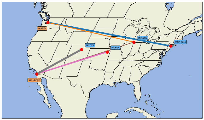
Now we have all the data we need in Python. We can now go ahead and analyse the data in any way we like, using the huge range of available Python packages. Below, we use Cartopy to plot amounts shipped between plants and markets, with thicker lines denoting a larger amount of goods to transport.

import matplotlib.pyplot as plt
import cartopy.crs as ccrs
import cartopy.feature as cfeature

fig = plt.figure(figsize=(15, 10))
ax = fig.add_subplot(1, 1, 1, projection=ccrs.Robinson())
ax.coastlines()
ax.set_extent([-125, -66.5, 20, 50], crs=ccrs.Geodetic())
ax.add_feature(cfeature.LAND)
ax.add_feature(cfeature.OCEAN)
ax.add_feature(cfeature.STATES)


for index, row in x.iterrows():
    p_loc = list(plant_locations[row.Plant])
    m_loc = list(market_locations[row.Market])
    w     = row.level / 50
    
    ax.plot([p_loc[1],m_loc[1]],[p_loc[0],m_loc[0]], transform=ccrs.PlateCarree(), linewidth=w)
    ax.plot(p_loc[1], p_loc[0], marker='o', color='red', markersize=12, transform=ccrs.PlateCarree())
    ax.plot(m_loc[1], m_loc[0], marker='o', color='red', markersize=12, transform=ccrs.PlateCarree())
    ax.text(p_loc[1] -2, p_loc[0] - 2, row.Plant, transform=ccrs.Geodetic(),
           bbox=dict(facecolor='sandybrown', boxstyle='round')) 
    ax.text(m_loc[1] +1, m_loc[0] + 1, row.Market, transform=ccrs.Geodetic(),
           bbox=dict(facecolor='#60b0f4', boxstyle='round')) 
    
plt.show()
    

Below is the listing of the geo.py module with the helper functions that calculate distances between cities.

from geopy.geocoders import Nominatim
from geopy.distance import geodesic
import time

def get_locations(cities):
    '''Retrieve geo location from OpenStreetMap data'''

    # Create a new client to resolve addresses to locations
    geo = Nominatim(user_agent="gamstransfer_example")
    
    locations = {}
    for city in cities:
        time.sleep(1)  # Limit the number of requests to the server
        loc = geo.geocode(city)
        locations[city] = (loc.latitude, loc.longitude)
        
    return locations


def calculate_distances(sources,destinations):
    ''' Calculate the distances for all city pairs'''
    
    distances = []
    for source,sourceLoc in sources.items():
        for dest, destLoc in destinations.items():
            distances.append((source,dest,0.001 * geodesic((sourceLoc[0],sourceLoc[1]),(destLoc[0],destLoc[1])).miles))
    return distances