Introduction

In the dynamic landscape of modern commerce, where competition is fierce and customer expectations are ever-evolving, the need for businesses to continuously optimize their operations has become paramount. Whether you’re a budding startup or an established enterprise, embracing the philosophy of optimization can be the difference between stagnation and sustainable growth.

In this blog post, we delve into the fundamental reasons why optimizing your business processes and resources is not just a luxury but a necessity for long-term success. From enhancing efficiency and maximizing productivity to minimizing cost and efficiently allocating resources, the benefits of optimization are multifaceted and far-reaching.

To get started, let’s delve into the example of painting cars in car manufacturing. This scenario serves as a practical illustration of the complexities involved in optimizing decisions, where efficiency and accuracy are paramount.

The Binary Paintshop Problem

In the complex world of car manufacturing, each step in the production process plays a crucial role in ensuring efficiency and quality. One such critical step is painting, where cars receive their final aesthetic touch before hitting the roads. Imagine a scenario where cars of different types (A to F) arrive on a conveyor belt at a paintshop in a specific sequence, as depicted in the diagram below:

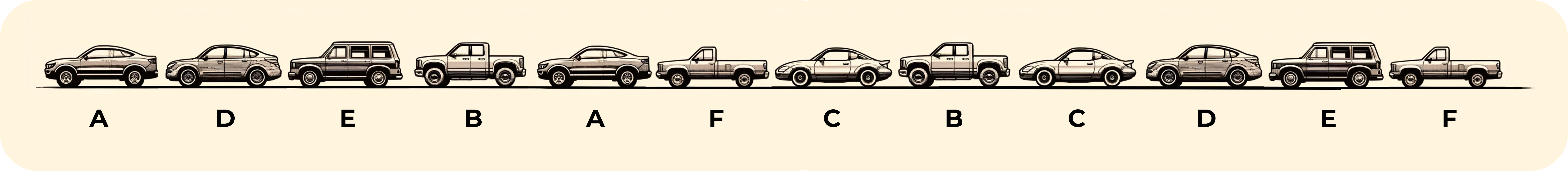
Each car needs to be painted with a base coat that can either be white or black.

To simplify this scenario, let’s consider a minimal working example:

• Each vehicle type (A to F) arrives exactly twice in the sequence.
• One car of each type must be painted white, while the other must be painted black.
• The order of the arriving cars cannot be adjusted.
• Changing the color consumes time and resources.

The objective here is to minimize the number of color changes while ensuring that each vehicle type receives both white and black paint.

This scenario encapsulates what is known as the Binary Paintshop Problem, a classic optimization problem that illustrates the challenges businesses face when trying to minimize resource usage while meeting specific constraints.

Your Turn

Now, imagine yourself in the driver’s seat, tasked with deciding which car receives a coat of white and which gets painted black. Grab a pair of pens with contrasting colors, and let’s dive into the challenge. Take the sequence of letters representing each car type and strategize how to color each letter with the fewest possible color changes, ensuring that every car type receives both white and black paint.

Most individuals I challenge with this task typically arrive at the same conclusion: four color changes are required. Here’s how they typically paint the cars:

Show solution

Now, you are tasked with explaining the solution process to a coworker to guide them through the challenge. Consider the steps they need to take to efficiently tackle the problem.

Here’s a common approach that most people I challenge with this task tend to formulate:

Algorithms and Heuristics

This approach is what we call a Greedy Algorithm or Greedy Heuristic. A greedy algorithm is a simple and intuitive approach to solving optimization problems. It makes a series of locally optimal choices at each step with the hope of finding a global optimum. In other words, at each step, it selects the best available option without considering the future consequences. Greedy algorithms are often fast and easy to implement, but they may not always produce the best solution for complex problems. Many companies already make use of similar approaches, especially when structuring tasks in Excel Workbooks or VBA macros, aiming for quick and practical solutions.

We can harness the power of the described greedy algorithm by implementing it, for instance, in Python. This allows us to efficiently apply the defined rules on how to color the arriving car types, even for larger sequences. By translating the problem-solving strategy into code, we can automate the process and expedite the optimization of resource usage.

changes = 0
colors = {"white": set(), "black": set()}
result = []


def paint_car(colors_dict, result_list, color, car_type):
    colors_dict[color].add(car_type)
    result_list.append(color)


current_color = "white"
for car in sequence:
    if car not in colors[current_color]:
        paint_car(colors, result, current_color, car)
    else:
        # change color
        changes += 1
        if current_color == "white":
            current_color = "black"
        else:
            current_color = "white"
        paint_car(colors, result, current_color, car)

Applying the code above to our ADEBAFCBCDEF sequence, we yield the expected four color changes.

>>> print(result)
['white', 'white', 'white', 'white', 'black', 'black', 'black', 'black', 'white', 'black', 'black', 'white']
>>> print("Number of changes:", changes)
Number of changes: 4

Mathematical Optimization

An alternative to heuristic solution approaches, such as the presented greedy algorithm, is mathematical optimization. With mathematical optimization we shift the perspective from prescribing rules to yield a solution towards precisely defining and describing the problem we try to solve. By formulating the problem mathematically, we can articulate the objective, constraints, and decision variables in a rigorous manner. This approach enables us to explore the problem space more systematically, leveraging mathematical techniques to identify optimal solutions efficiently.

Below, you will find the mathematical representation of the Binary Paintshop Problem, for which we’ve devised the greedy algorithm:

$$\min F = \sum_{i \in \mathcal{I} \hspace{0.75mm} | \hspace{0.75mm} i < |I|} (X_i - X_{i+1})^2 \tag{1} $$

$$ \sum_{i: (i,j) \in \mathcal{IJ}} X_i = 1 \hspace{1cm} \forall \ j \in \mathcal{J} \tag{2} $$

$$ X_i \in \lbrace 0, 1\rbrace \hspace{1cm} \forall \ (i,j) \in \mathcal{IJ} \tag{3} $$

To understand the importance of mathematical optimization especially compared to using heuristic approaches, you don’t need to read or even understand the details of the mathematical model and you can directly skip to the results . However, if you are interested in the model formulation, here is a brief explanation.

As a preliminary step, we introduce two distinct sets: $\mathcal{I}$ and $\mathcal{J}$. Set $\mathcal{I}$ contains all positions within our sequence, numbered sequentially, while set $\mathcal{J}$ comprises each unique vehicle type, represented by letters A to F.

To define the order of vehicle type arrivals at the paintshop, we introduce the set $(i,j) \in \mathcal{IJ}$. Each element in this set corresponds to a specific position $i$ in the sequence, indicating which vehicle type $j \in \mathcal{j}$ arrives at that point. For our ADEBAFCBCDEF sequence, $(1,A):\mathcal{IJ}$ represents car type $j=A$ arriving at position $i=1$, and $(2,D):\mathcal{IJ}$ specifies car type $j=D$ arriving at position $i=2$, and so forth.

Within our mathematical notation, $X_i$ embodies the core decision-making process. It represents the choice regarding the color used at position $i \in \mathcal{I}$ within our sequence. For instance, $X_3 = 1$ signifies painting the vehicle at position 3 black, while $X_3 = 0$ indicates using white.

The fundamental rule governing our paintshop problem dictates that each vehicle type $j \in \mathcal{J}$ must be painted black exactly once. Thus, for every vehicle type $j \in \mathcal{J}$, we sum over all $X_i$ across $(i,j) \in \mathcal{IJ}$ and enforce this sum to be exactly one, ensuring adherence to the rule and represented by Equation (2). For example, for the sequence ADEBAFCBCDEF, the equations derived from this rule would appear as follows:

$$ \text{Equation (2)}_A: X_1 + X_5 = 1 $$ $$ \text{Equation (2)}_B: X_4 + X_8 = 1 $$ $$ \text{Equation (2)}_C: X_7 + X_9 = 1 $$ $$ \text{Equation (2)}_D: X_2 + X_10 = 1 $$ $$ \text{Equation (2)}_E: X_3 + X_11 = 1 $$ $$ \text{Equation (2)}_F: X_6 + X_12 = 1 $$

To establish our objective, we aim to minimize the number of color changes within our sequence. This objective is achieved by examining each position $i \in \mathcal{I}$ in our sequence and assessing whether its successor $i+1$ refers to a different color, as outlined in Equation (1). When the difference $X_i−X_{i+1}$ equals $1$ or $-1$, it signifies a change in color, incrementing our objective by one. Conversely, a difference of zero indicates no color change.

Our overarching aim is to minimize the total number of color changes, thus necessitating the definition of our objective as a minimization function.

With a precise mathematical representation of the problem, we can utilize off-the-shelf optimization solvers to solve our paintshop problem with mathematically proven optimality, which ensures that no superior solution exists within the constraints of our problem.

Optimal solution

Upon solving the optimization problem, we obtain the optimal number of color changes, resulting in a value of two in our example. Additionally, we derive optimal values for our decision variables $X_i$ leading to the following colored sequence:

Transitioning to Real-world Challenges: The Multi-Vehicle Paintshop Problem

In my experience presenting the Binary Paintshop Problem to a broader audience, there’s often someone astute enough to start coloring the given sequence from the back, ultimately arriving at the optimal solution of two color changes. This observation offers valuable insight: when tackling problems heuristically, where the approach to reaching a solution is specified, there can be multiple viable pathways to a solution. Moreover, these solutions can vary significantly from one another. However, the crucial question remains:

How do we discern the most effective approach to reaching a solution?

It’s important to note that starting from the back only proves efficacious for this particular sequence.

Also, it is crucial to remember that the example discussed here serves as a simplification of a real-world problem. In reality, we deal with a larger sequence of arriving car types, where each type may arrive any number of times. Additionally, we must accommodate specific demands regarding the number of cars of each type that need to be painted both white and black.

We can easily adapt our Greedy algorithm to account for specific color demands:

changes = 0
colors = {"white": dict(demand_white), "black": dict(demand_black)}
result = []


def paint_car(colors_dict, result_list, color, car_type):
    colors_dict[color][car_type] -= 1
    result_list.append(color)


current_color = "white"
for car in sequence:
    if colors[current_color][car] > 0:
        paint_car(colors, result, current_color, car)
    else:
        # change color
        changes += 1
        if current_color == "white":
            current_color = "black"
        else:
            current_color = "white"
        paint_car(colors, result, current_color, car)

Running the above code for a random sequence of arriving car types of length 128 results in a coloring with 31 color changes.

>>> print("Number of changes:", changes)
Number of changes: 31

Now, let’s proceed to adapt our mathematical model to accommodate these real-world complexities.

$$\min F = \sum_{i \in \mathcal{I} \hspace{0.75mm} | \hspace{0.75mm} i < |I|} (X_i - X_{i+1})^2 \tag{4} $$

$$ \sum_{i: (i,j) \in \mathcal{IJ}} 1 X_i = d^{black}_j \hspace{1cm} \forall \ j \in \mathcal{J} \tag{5} $$

$$ \sum_{i: (i,j) \in \mathcal{IJ}} 1 - X_i = d^{white}_j \hspace{1cm} \forall \ j \in \mathcal{J} \tag{6} $$

$$ X_i \in \lbrace 0, 1\rbrace \hspace{1cm} \forall \ (i,j) \in \mathcal{IJ} \tag{7} $$

It’s worth noting that we retain the same objective function (Equation (1) is the same as Equation (4)) in our adapted mathematical model. However, to accommodate the color demands, we introduce two new constraints. Firstly, by replacing the equality constraint in Equation (2) with the demand for black-colored car types in Equation (5), we ensure that exactly $d^{black}_j$ vehicles are painted black. Secondly, to address the demand for white cars, we employ a similar equation as for black cars (Equation (6)), but sum over $1−X_i$.

Upon solving our adapted model we arrive at a solution requiring only 11 color changes.

>>> print("Number of changes:", changes)
Number of changes: 11

Through the utilization of mathematical optimization in our example, we’ve observed significant improvements in decision-making regarding color changes. This enhancement translates to reduced time required for color changes, improved resource utilization, and potentially lowered costs or increased productivity within a given time frame.

Transfer to Other Problem Types

Expanding beyond the realm of the Binary Paintshop Problem, mathematical optimization demonstrates its efficacy across various problem types. While the problem we’ve discussed is relatively straightforward, mathematical optimization empowers us to tackle large and intricate real-world problems effectively. Its applications span across diverse fields, including agriculture, logistics, scheduling, energy systems, and many more.

Do you encounter such complex problems in your domain? Feel free to reach out to consulting@gams.com for assistance in finding optimized solutions tailored to your specific needs. A Jupyter Notebook with all relevant code snippets can be accessed here .