From GAMSPy Model to GAMS MIRO App

In this tutorial, we will explore the powerful features of GAMS MIRO to generate an application tailored to your optimization problem. Step by step, we will build the MIRO application for this gallery example.

To be able to follow this tutorial, we assume that you have already worked with GAMS or GAMSPy, as we will start with a given GAMSPy model. The content of the first section is GAMSPy specific, everything after that applies to both GAMS and GAMSPy. So if you are working with a GAMS model, you can check the documentation for the syntax, still it might be helpful to follow the tutorial for additional explanations. Otherwise, you just need to have MIRO installed (this tutorial is based on version 2.12.0, if you are using an older version, some of the features we will go through may be missing), and some R knowledge might help in the third part of the tutorial, but is not required. All necessary R functions will be explained, so if you have worked with a similar language before, you are good to go!

As already mentioned, you can start with either a GAMS or a GAMSPy implementation; we’ll be working with a GAMSPy model. Our first step will be to define the application’s inputs and outputs - this is the only part of the process that differs depending on whether you are using GAMS or GAMSPy. After that, the configuration process is the same for both.

We’ll start by showing you how to specify inputs and outputs in your GAMSPy model. Then we will see how to visualize data in MIRO using only these definitions. This step can be extremely helpful during model development: it allows you to quickly plot and inspect the output data to make sure your results make sense. If something doesn’t look right, you have a clear starting point for investigating potential errors in you model implementation.

After we’ve covered the basics of visualization, in the second part of this tutorial we’ll move on to the Configuration Mode. Here you can configure many default settings without editing any code, making it easy to customize your application for different needs. Since built-in options are sometimes not enough, the third part of this tutorial will show you how to add custom renderers and widgets to give you maximum control over the user interface. Finally, we’ll examine advanced customization tips and tricks that can make your MIRO application even more powerful and tailored to your needs.

From GAMSPy Model to GAMS MIRO App

Implement the Model

The starting point for building your MIRO application is the implementation of your model using either GAMS or GAMSPy. As mentioned, we will be using a GAMSPy model here. If you would like to see how the necessary code modifications would look in GAMS, please refer to the documentation .

Our example model is a “Battery Energy Storage System (BESS) sizing problem,” based on an example from NAG , available on their GitHub (BESS.ipynb ). The goal is to optimize a city’s hourly energy schedule by identifying the most cost-effective combination of energy sources, which includes leveraging a BESS to store low-cost energy during off-peak hours and release it when demand is high. By assessing different storage capacities and discharge rates, the model pinpoints the configuration that minimizes overall energy costs while ensuring demand is consistently met.

Before diving in, we recommend that you review the mathematical description in the introduction to the finished application provided in the gallery . We will be referring directly to the variable names introduced there.

GAMSPy model code

import pandas as pd
import sys

from gamspy import (
    Container,
    Alias,
    Equation,
    Model,
    Parameter,
    Sense,
    Set,
    Sum,
    Variable,
    Ord,
    Options,
    ModelStatus,
    SolveStatus,
)


def main():
    m = Container()

    # Generator parameters
    generator_specifications_input = pd.DataFrame(
        [
            ["gen0", 1.1, 220, 50, 100, 4, 2],
            ["gen1", 1.3, 290, 80, 190, 4, 2],
            ["gen2", 0.9, 200, 10, 70, 4, 2],
        ],
        columns=[
            "i",
            "cost_per_unit",
            "fixed_cost",
            "min_power_output",
            "max_power_output",
            "min_up_time",
            "min_down_time",
        ],
    )

    # Load demand to be fulfilled by the energy management system
    # combine with cost external grid, to have one source of truth for the hours (Set j)
    timewise_load_demand_and_cost_external_grid_input = pd.DataFrame(
        [
            ["hour00", 200, 1.5],
            ["hour01", 180, 1.0],
            ["hour02", 170, 1.0],
            ["hour03", 160, 1.0],
            ["hour04", 150, 1.0],
            ["hour05", 170, 1.0],
            ["hour06", 190, 1.2],
            ["hour07", 210, 1.8],
            ["hour08", 290, 2.1],
            ["hour09", 360, 1.9],
            ["hour10", 370, 1.8],
            ["hour11", 350, 1.6],
            ["hour12", 310, 1.6],
            ["hour13", 340, 1.6],
            ["hour14", 390, 1.8],
            ["hour15", 400, 1.9],
            ["hour16", 420, 2.1],
            ["hour17", 500, 3.0],
            ["hour18", 440, 2.1],
            ["hour19", 430, 1.9],
            ["hour20", 420, 1.8],
            ["hour21", 380, 1.6],
            ["hour22", 340, 1.2],
            ["hour23", 320, 1.2],
        ],
        columns=["j", "load_demand", "cost_external_grid"],
    )

    # Set
    i = Set(
        m,
        name="i",
        records=generator_specifications_input["i"],
        description="generators",
    )
    j = Set(
        m,
        name="j",
        records=timewise_load_demand_and_cost_external_grid_input["j"],
        description="hours",
    )
    t = Alias(m, name="t", alias_with=j)

    # Data
    # Generator parameters
    gen_cost_per_unit = Parameter(
        m,
        name="gen_cost_per_unit",
        domain=[i],
        records=generator_specifications_input[["i", "cost_per_unit"]],
        description="cost per unit of generator i",
    )

    gen_fixed_cost = Parameter(
        m,
        name="gen_fixed_cost",
        domain=[i],
        records=generator_specifications_input[["i", "fixed_cost"]],
        description="fixed cost of generator i",
    )

    gen_min_power_output = Parameter(
        m,
        name="gen_min_power_output",
        domain=[i],
        records=generator_specifications_input[["i", "min_power_output"]],
        description="minimal power output of generator i",
    )

    gen_max_power_output = Parameter(
        m,
        name="gen_max_power_output",
        domain=[i],
        records=generator_specifications_input[["i", "max_power_output"]],
        description="maximal power output of generator i",
    )

    gen_min_up_time = Parameter(
        m,
        name="gen_min_up_time",
        domain=[i],
        records=generator_specifications_input[["i", "min_up_time"]],
        description="minimal up time of generator i",
    )

    gen_min_down_time = Parameter(
        m,
        name="gen_min_down_time",
        domain=[i],
        records=generator_specifications_input[["i", "min_down_time"]],
        description="minimal down time of generator i",
    )

    # Battery parameters
    cost_bat_power = Parameter(m, "cost_bat_power", records=1, is_miro_input=True)
    cost_bat_energy = Parameter(m, "cost_bat_energy", records=2, is_miro_input=True)

    # Load demand and external grid
    load_demand = Parameter(
        m, name="load_demand", domain=[j], description="load demand at hour j"
    )

    cost_external_grid = Parameter(
        m,
        name="cost_external_grid",
        domain=[j],
        description="cost of the external grid at hour j",
    )

    max_input_external_grid = Parameter(
        m,
        name="max_input_external_grid",
        records=10,
        description="maximal power that can be imported from the external grid every hour",
    )

    # Variable
    # Generator
    gen_power = Variable(
        m,
        name="gen_power",
        type="positive",
        domain=[i, j],
        description="Dispatched power from generator i at hour j",
    )

    gen_active = Variable(
        m,
        name="gen_active",
        type="binary",
        domain=[i, j],
        description="is generator i active at hour j",
    )

    # Battery
    battery_power = Variable(
        m,
        name="battery_power",
        domain=[j],
        description="power charged or discharged from the battery at hour j",
    )

    battery_delivery_rate = Variable(
        m,
        name="battery_delivery_rate",
        description="power (delivery) rate of the battery energy system",
    )

    battery_storage = Variable(
        m,
        name="battery_storage",
        description="energy (storage) rate of the battery energy system",
    )

    # External grid
    external_grid_power = Variable(
        m,
        name="external_grid_power",
        type="positive",
        domain=[j],
        description="power imported from the external grid at hour j",
    )

    # Equation
    fulfill_load = Equation(
        m,
        name="fulfill_load",
        domain=[j],
        description="load balance needs to be met very hour j",
    )

    gen_above_min_power = Equation(
        m,
        name="gen_above_min_power",
        domain=[i, j],
        description="generators power should be above the minimal output",
    )

    gen_below_max_power = Equation(
        m,
        name="gen_below_max_power",
        domain=[i, j],
        description="generators power should be below the maximal output",
    )

    gen_above_min_down_time = Equation(
        m,
        name="gen_above_min_down_time",
        domain=[i, j],
        description="generators down time should be above the minimal down time",
    )

    gen_above_min_up_time = Equation(
        m,
        name="gen_above_min_up_time",
        domain=[i, j],
        description="generators up time should be above the minimal up time",
    )

    battery_above_min_delivery = Equation(
        m,
        name="battery_above_min_delivery",
        domain=[j],
        description="battery delivery rate (charge rate) above min power rate",
    )

    battery_below_max_delivery = Equation(
        m,
        name="battery_below_max_delivery",
        domain=[j],
        description="battery delivery rate below max power rate",
    )

    battery_above_min_storage = Equation(
        m,
        name="battery_above_min_storage",
        domain=[t],
        description="battery storage above negative energy rate (since negative power charges the battery)",
    )

    battery_below_max_storage = Equation(
        m,
        name="battery_below_max_storage",
        domain=[t],
        description="sum over battery delivery below zero (cant deliver energy that is not stored)",
    )

    external_power_upper_limit = Equation(
        m,
        name="external_power_upper_limit",
        domain=[j],
        description=" input from the external grid is limited",
    )

    fulfill_load[j] = (
        Sum(i, gen_power[i, j]) + battery_power[j] + external_grid_power[j]
        == load_demand[j]
    )

    gen_above_min_power[i, j] = (
        gen_min_power_output[i] * gen_active[i, j] <= gen_power[i, j]
    )

    gen_below_max_power[i, j] = (
        gen_power[i, j] <= gen_max_power_output[i] * gen_active[i, j]
    )

    # if j=0 -> j.lag(1) = 0 which doesn't brake the equation,
    # since generator is of at start, resulting in negative right side, therefore the sum is always above
    gen_above_min_down_time[i, j] = Sum(
        t.where[(Ord(t) >= Ord(j)) & (Ord(t) <= (Ord(j) + gen_min_down_time[i] - 1))],
        1 - gen_active[i, t],
    ) >= gen_min_down_time[i] * (gen_active[i, j.lag(1)] - gen_active[i, j])

    # and for up it correctly starts the check that if its turned on in the first step
    # it has to stay on for the min up time
    gen_above_min_up_time[i, j] = Sum(
        t.where[(Ord(t) >= Ord(j)) & (Ord(t) <= (Ord(j) + gen_min_up_time[i] - 1))],
        gen_active[i, t],
    ) >= gen_min_up_time[i] * (gen_active[i, j] - gen_active[i, j.lag(1)])

    battery_above_min_delivery[j] = -battery_delivery_rate <= battery_power[j]

    battery_below_max_delivery[j] = battery_power[j] <= battery_delivery_rate

    battery_above_min_storage[t] = -battery_storage <= Sum(
        j.where[Ord(j) <= Ord(t)], battery_power[j]
    )

    battery_below_max_storage[t] = Sum(j.where[Ord(j) <= Ord(t)], battery_power[j]) <= 0

    external_power_upper_limit[j] = external_grid_power[j] <= max_input_external_grid

    obj = (
        Sum(
            j,
            Sum(i, gen_cost_per_unit[i] * gen_power[i, j] + gen_fixed_cost[i])
            + cost_external_grid[j] * external_grid_power[j],
        )
        + cost_bat_power * battery_delivery_rate
        + cost_bat_energy * battery_storage
    )

    # Solve
    bess = Model(
        m,
        name="bess",
        equations=m.getEquations(),
        problem="MIP",
        sense=Sense.MIN,
        objective=obj,
    )

    bess.solve(
        solver="CPLEX",
        output=sys.stdout,
        options=Options(equation_listing_limit=1, relative_optimality_gap=0),
    )

    if bess.solve_status not in [
        SolveStatus.NormalCompletion,
        SolveStatus.TerminatedBySolver,
    ] or bess.status not in [ModelStatus.OptimalGlobal, ModelStatus.Integer]:
        print("No solution exists for your input data.\n")
        raise Exception("Infeasible.")

if __name__ == "__main__":
    main()

Model Input

Let’s start by defining some basic inputs. You can see that we begin with three scalar parameters, each of which has the additional is_miro_input=True option in the definition:

# Battery parameters
cost_bat_power = Parameter(m, "cost_bat_power", records=1, is_miro_input=True)
cost_bat_energy = Parameter(m, "cost_bat_energy", records=2, is_miro_input=True)

# Load demand and external grid
max_input_external_grid = Parameter(
    m,
    name="max_input_external_grid",
    records=10,
    is_miro_input=True,
    description="maximal power that can be imported from the external grid every hour",
)

For the generator specifications and schedule inputs, there are a few extra steps. The model relies on two sets: one for possible generators and another for hours in which load demand must be met. Since these sets are not fixed but should be part of the input, we use Domain Forwarding - an approach where the set is implicitly defined by one parameter.

Because multiple parameters rely on these sets and we want a single source of truth, we need to combine them into a single table in our MIRO application (one for generator specifications, another for the schedule). To achieve this, we define an additional set for the column headers:


generator_spec_header = Set(
    m,
    name="generator_spec_header",
    records=[
        "cost_per_unit",
        "fixed_cost",
        "min_power_output",
        "max_power_output",
        "min_up_time",
        "min_down_time",
    ],
)

We then create a parameter to hold all the relevant information:

generator_specifications = Parameter(
    m,
    name="generator_specifications",
    domain=[i, generator_spec_header],
    domain_forwarding=[True, False],
    records=generator_specifications_input.melt(
        id_vars="i", var_name="generator_spec_header"
    ),
    is_miro_input=True,
    is_miro_table=True,
    description="specifications of each generator",
)

Notice that is_miro_input=True makes the parameter an input to the MIRO application, while is_miro_table=True displays the data in table format . The key detail is domain_forwarding=[True, False], which ensures that set elements for generators come from the MIRO application (the header names remain fixed, hence False). We still use our initial data to populate these specifications, but we transform it using melt() so that it matches the new format of only two columns: "i" and "generator_spec_header".

Since we are now forwarding the domain of set i through this table, we no longer specify its records. The same goes for any parameters that rely on i (e.g., gen_cost_per_unit). Instead, we assign them by referencing the new combined parameter:

i = Set(
    m,
    name="i",
-   records=generator_specifications_input["i"],
    description="generators",
)

gen_cost_per_unit = Parameter(
      m,
      name="gen_cost_per_unit",
      domain=[i],
-     records=generator_specifications_input[["i", "cost_per_unit"]],
      description="cost per unit of generator i",
  )

+ gen_cost_per_unit[i] = generator_specifications[i, "cost_per_unit"]

We apply the same pattern to other parameters that depend on i. Likewise, for hour-dependent parameters (like load_demand and cost_external_grid), we create a single source of truth for the hour set by combining them into one parameter and making the same modifications.

Given the input, we move on to the output.

Model Output

When implementing the model, it can be helpful to flag variables as outputs by adding is_miro_output=True. After solving, we can then view the calculated variable values right away, making it easier to spot any remaining model errors.

gen_power = Variable(
    m,
    name="gen_power",
    type="positive",
    domain=[i, j],
    description="dispatched power from generator i at hour j",
    is_miro_output=True,
)

In general, we can designate any variable or parameter as an MIRO output. When implementing the model, it makes sense to simply define all variables as output, so you can easily visualize the results. Sometimes it makes sense to define parameters as outputs that depend on the variables. A straightforward example in our model is to create dedicated parameters for the three cost components, allowing us to display these values directly in the MIRO application:

total_cost_gen = Parameter(
    m,
    "total_cost_gen",
    is_miro_output=True,
    description="total cost of the generators",
)

total_cost_gen[...] = Sum(
    j, Sum(i, gen_cost_per_unit[i] * gen_power.l[i, j] + gen_fixed_cost[i])
)

We apply this same approach for the other power sources and combine them:

Costs for the other power sources

total_cost_battery = Parameter(
    m,
    "total_cost_battery",
    is_miro_output=True,
    description="total cost of the BESS",
)

total_cost_battery[...] = (
    cost_bat_power * battery_delivery_rate.l + cost_bat_energy * battery_storage.l
)

total_cost_extern = Parameter(
    m,
    "total_cost_extern",
    is_miro_output=True,
    description="total cost for the imported power",
)

total_cost_extern[...] = Sum(
    j,
    cost_external_grid[j] * external_grid_power.l[j],
)

total_cost = Parameter(
    m,
    "total_cost",
    is_miro_output=True,
    description="total cost to fulfill the load demand",
)

total_cost[...] = total_cost_gen + total_cost_battery + total_cost_extern

We also combine our power variables with the load demand input into a single output parameter to later show how the sum of all power flows meets the load demand:

# Power output
power_output_header = Set(
    m,
    name="power_output_header",
    records=["battery", "external_grid", "generators", "load_demand"],
)

report_output = Parameter(
    m,
    name="report_output",
    domain=[j, power_output_header],
    description="optimal combination of incoming power flows",
    is_miro_output=True,
)

report_output[j, "generators"] = Sum(i, gen_power.l[i, j])
report_output[j, "battery"] = battery_power.l[j]
report_output[j, "external_grid"] = external_grid_power.l[j]
report_output[j, "load_demand"] = load_demand[j]

Now, we can launch MIRO to see our first fully interactive modeling application!

gamspy run miro --path <path_to_your_MIRO_installation> --model <path_to_your_model>

After starting MIRO, the application should look like this:

Effective Data Validation Using Log Files

Finally, we will briefly discuss data validation. This is critical to ensuring the accuracy and reliability of optimization models. Log files are key to checking the consistency of input data, and generating reports on inconsistencies helps prevent errors and user frustration. Here we will only verify that our input values are all non-negative. While finding effective validation checks can be challenging, clearly identifying the constraints or values causing infeasibility can significantly improve the user experience.

In MIRO, you have the option to create a custom log file. However, since we are using GAMSPy, we can also directly write to stdout and log there. And if we here follow the specified MIRO log syntax , here any invalid data can be highlighted directly above the corresponding input data sheet in MIRO.

The syntax that must be used for MIRO to jump directly to the table with the incorrect data is as follows:

symbolname:: Error message

Try for yourself how a simple verification of the sign of the input values might look. Keep in mind that you should validate the data before attempting to solve the model. If the validation fails, specify which value caused the failure and raise an exception, as there’s no need to solve the model in this case.

A possible data validation

no_negative_gen_spec = generator_specifications.records[generator_specifications.records["value"] < 0]
no_negative_load = load_demand.records[load_demand.records["value"] < 0]
no_negative_cost = cost_external_grid.records[
    cost_external_grid.records["value"] < 0
]

print(
    """------------------------------------\n       Validating data\n------------------------------------\n"""
)
errors = False

if not no_negative_gen_spec.empty:
    print(
        "generator_specifications:: No negative values for the generator specifications allowed!\n"
    )
    for _, row in no_negative_gen_spec.iterrows():
        print(f'{row["i"]} has a negative value.\n')
    errors = True

if not no_negative_load.empty:
    print(
        "timewise_load_demand_and_cost_external_grid_data:: No negative load demand allowed!\n"
    )
    for _, row in no_negative_load.iterrows():
        print(f'{row["j"]} has negative load demand.\n')
    errors = True

if not no_negative_cost.empty:
    print(
        "timewise_load_demand_and_cost_external_grid_data:: No negative cost allowed!\n"
    )
    for _, row in no_negative_cost.iterrows():
        print(f'{row["j"]} has negative external grid cost.\n')
    errors = True

if errors:
    raise Exception("Data errors detected")
print("Data ok\n")

Full updated GAMSPy model

import pandas as pd
import sys

from gamspy import (
    Container,
    Alias,
    Equation,
    Model,
    Parameter,
    Sense,
    Set,
    Sum,
    Variable,
    Ord,
    Options,
    ModelStatus,
    SolveStatus,
)


def main():
    m = Container()

    # Generator parameters
    generator_specifications_input = pd.DataFrame(
        [
            ["gen0", 1.1, 220, 50, 100, 4, 2],
            ["gen1", 1.3, 290, 80, 190, 4, 2],
            ["gen2", 0.9, 200, 10, 70, 4, 2],
        ],
        columns=[
            "i",
            "cost_per_unit",
            "fixed_cost",
            "min_power_output",
            "max_power_output",
            "min_up_time",
            "min_down_time",
        ],
    )

    # Load demand to be fulfilled by the energy management system
    # combine with cost external grid, to have one source of truth for the hours (Set j)
    timewise_load_demand_and_cost_external_grid_input = pd.DataFrame(
        [
            ["hour00", 200, 1.5],
            ["hour01", 180, 1.0],
            ["hour02", 170, 1.0],
            ["hour03", 160, 1.0],
            ["hour04", 150, 1.0],
            ["hour05", 170, 1.0],
            ["hour06", 190, 1.2],
            ["hour07", 210, 1.8],
            ["hour08", 290, 2.1],
            ["hour09", 360, 1.9],
            ["hour10", 370, 1.8],
            ["hour11", 350, 1.6],
            ["hour12", 310, 1.6],
            ["hour13", 340, 1.6],
            ["hour14", 390, 1.8],
            ["hour15", 400, 1.9],
            ["hour16", 420, 2.1],
            ["hour17", 500, 3.0],
            ["hour18", 440, 2.1],
            ["hour19", 430, 1.9],
            ["hour20", 420, 1.8],
            ["hour21", 380, 1.6],
            ["hour22", 340, 1.2],
            ["hour23", 320, 1.2],
        ],
        columns=["j", "load_demand", "cost_external_grid"],
    )

    # Set
    i = Set(
        m,
        name="i",
        description="generators",
    )
    j = Set(
        m,
        name="j",
        description="hours",
    )
    t = Alias(m, name="t", alias_with=j)

    generator_spec_header = Set(
        m,
        name="generator_spec_header",
        records=[
            "cost_per_unit",
            "fixed_cost",
            "min_power_output",
            "max_power_output",
            "min_up_time",
            "min_down_time",
        ],
    )

    timewise_header = Set(
        m, name="timewise_header", records=["load_demand", "cost_external_grid"]
    )

    # Data
    # Generator parameters
    generator_specifications = Parameter(
        m,
        name="generator_specifications",
        domain=[i, generator_spec_header],
        domain_forwarding=[True, False],
        records=generator_specifications_input.melt(
            id_vars="i", var_name="generator_spec_header"
        ),
        is_miro_input=True,
        is_miro_table=True,
        description="Specifications of each generator",
    )

    # To improve readability of the equations we extract the individual columns.
    # Since we want a single source of truth we combine them for MIRO.
    gen_cost_per_unit = Parameter(
        m,
        name="gen_cost_per_unit",
        domain=[i],
        description="cost per unit of generator i",
    )

    gen_fixed_cost = Parameter(
        m, name="gen_fixed_cost", domain=[i], description="fixed cost of generator i"
    )

    gen_min_power_output = Parameter(
        m,
        name="gen_min_power_output",
        domain=[i],
        description="minimal power output of generator i",
    )

    gen_max_power_output = Parameter(
        m,
        name="gen_max_power_output",
        domain=[i],
        description="maximal power output of generator i",
    )

    gen_min_up_time = Parameter(
        m,
        name="gen_min_up_time",
        domain=[i],
        description="minimal up time of generator i",
    )

    gen_min_down_time = Parameter(
        m,
        name="gen_min_down_time",
        domain=[i],
        description="minimal down time of generator i",
    )

    gen_cost_per_unit[i] = generator_specifications[i, "cost_per_unit"]
    gen_fixed_cost[i] = generator_specifications[i, "fixed_cost"]
    gen_min_power_output[i] = generator_specifications[i, "min_power_output"]
    gen_max_power_output[i] = generator_specifications[i, "max_power_output"]
    gen_min_up_time[i] = generator_specifications[i, "min_up_time"]
    gen_min_down_time[i] = generator_specifications[i, "min_down_time"]

    # Battery parameters
    cost_bat_power = Parameter(m, "cost_bat_power", records=1, is_miro_input=True)
    cost_bat_energy = Parameter(m, "cost_bat_energy", records=2, is_miro_input=True)

    # Load demand and external grid
    timewise_load_demand_and_cost_external_grid_data = Parameter(
        m,
        name="timewise_load_demand_and_cost_external_grid_data",
        domain=[j, timewise_header],
        domain_forwarding=[True, False],
        records=timewise_load_demand_and_cost_external_grid_input.melt(
            id_vars="j", var_name="timewise_header"
        ),
        is_miro_input=True,
        is_miro_table=True,
        description="Timeline for load demand and cost of the external grid.",
    )

    load_demand = Parameter(
        m, name="load_demand", domain=[j], description="load demand at hour j"
    )

    cost_external_grid = Parameter(
        m,
        name="cost_external_grid",
        domain=[j],
        description="cost of the external grid at hour j",
    )

    load_demand[j] = timewise_load_demand_and_cost_external_grid_data[j, "load_demand"]
    cost_external_grid[j] = timewise_load_demand_and_cost_external_grid_data[
        j, "cost_external_grid"
    ]

    max_input_external_grid = Parameter(
        m,
        name="max_input_external_grid",
        records=10,
        is_miro_input=True,
        description="maximal power that can be imported from the external grid every hour",
    )

    no_negative_gen_spec = generator_specifications.records[
        generator_specifications.records["value"] < 0
    ]
    no_negative_load = load_demand.records[load_demand.records["value"] < 0]
    no_negative_cost = cost_external_grid.records[
        cost_external_grid.records["value"] < 0
    ]

    print(
        """------------------------------------\n       Validating data\n------------------------------------\n"""
    )
    errors = False

    if not no_negative_gen_spec.empty:
        print(
            "generator_specifications:: No negative values for the generator specifications allowed!\n"
        )
        for _, row in no_negative_gen_spec.iterrows():
            print(f'{row["i"]} has a negative value.\n')
        errors = True

    if not no_negative_load.empty:
        print(
            "timewise_load_demand_and_cost_external_grid_data:: No negative load demand allowed!\n"
        )
        for _, row in no_negative_load.iterrows():
            print(f'{row["j"]} has negative load demand.\n')
        errors = True

    if not no_negative_cost.empty:
        print(
            "timewise_load_demand_and_cost_external_grid_data:: No negative cost allowed!\n"
        )
        for _, row in no_negative_cost.iterrows():
            print(f'{row["j"]} has negative external grid cost.\n')
        errors = True

    if errors:
        raise Exception("Data errors detected")
    print("Data ok\n")

    # Variable
    # Generator
    gen_power = Variable(
        m,
        name="gen_power",
        type="positive",
        domain=[i, j],
        description="Dispatched power from generator i at hour j",
        is_miro_output=True,
    )

    gen_active = Variable(
        m,
        name="gen_active",
        type="binary",
        domain=[i, j],
        description="is generator i active at hour j",
    )

    # Battery
    battery_power = Variable(
        m,
        name="battery_power",
        domain=[j],
        description="power charged or discharged from the battery at hour j",
        is_miro_output=True,
    )

    battery_delivery_rate = Variable(
        m,
        name="battery_delivery_rate",
        description="power (delivery) rate of the battery energy system",
        is_miro_output=True,
    )

    battery_storage = Variable(
        m,
        name="battery_storage",
        description="energy (storage) rate of the battery energy system",
        is_miro_output=True,
    )

    # External grid
    external_grid_power = Variable(
        m,
        name="external_grid_power",
        type="positive",
        domain=[j],
        description="power imported from the external grid at hour j",
        is_miro_output=True,
    )

    # Equation
    fulfill_load = Equation(
        m,
        name="fulfill_load",
        domain=[j],
        description="load balance needs to be met very hour j",
    )

    gen_above_min_power = Equation(
        m,
        name="gen_above_min_power",
        domain=[i, j],
        description="generators power should be above the minimal output",
    )

    gen_below_max_power = Equation(
        m,
        name="gen_below_max_power",
        domain=[i, j],
        description="generators power should be below the maximal output",
    )

    gen_above_min_down_time = Equation(
        m,
        name="gen_above_min_down_time",
        domain=[i, j],
        description="generators down time should be above the minimal down time",
    )

    gen_above_min_up_time = Equation(
        m,
        name="gen_above_min_up_time",
        domain=[i, j],
        description="generators up time should be above the minimal up time",
    )

    battery_above_min_delivery = Equation(
        m,
        name="battery_above_min_delivery",
        domain=[j],
        description="battery delivery rate (charge rate) above min power rate",
    )

    battery_below_max_delivery = Equation(
        m,
        name="battery_below_max_delivery",
        domain=[j],
        description="battery delivery rate below max power rate",
    )

    battery_above_min_storage = Equation(
        m,
        name="battery_above_min_storage",
        domain=[t],
        description="battery storage above negative energy rate (since negative power charges the battery)",
    )

    battery_below_max_storage = Equation(
        m,
        name="battery_below_max_storage",
        domain=[t],
        description="sum over battery delivery below zero (cant deliver energy that is not stored)",
    )

    external_power_upper_limit = Equation(
        m,
        name="external_power_upper_limit",
        domain=[j],
        description=" input from the external grid is limited",
    )

    fulfill_load[j] = (
        Sum(i, gen_power[i, j]) + battery_power[j] + external_grid_power[j]
        == load_demand[j]
    )

    gen_above_min_power[i, j] = (
        gen_min_power_output[i] * gen_active[i, j] <= gen_power[i, j]
    )

    gen_below_max_power[i, j] = (
        gen_power[i, j] <= gen_max_power_output[i] * gen_active[i, j]
    )

    # if j=0 -> j.lag(1) = 0 which doesn't brake the equation,
    # since generator is of at start, resulting in negative right side, therefore the sum is always above
    gen_above_min_down_time[i, j] = Sum(
        t.where[(Ord(t) >= Ord(j)) & (Ord(t) <= (Ord(j) + gen_min_down_time[i] - 1))],
        1 - gen_active[i, t],
    ) >= gen_min_down_time[i] * (gen_active[i, j.lag(1)] - gen_active[i, j])

    # and for up it correctly starts the check that if its turned on in the first step
    # it has to stay on for the min up time
    gen_above_min_up_time[i, j] = Sum(
        t.where[(Ord(t) >= Ord(j)) & (Ord(t) <= (Ord(j) + gen_min_up_time[i] - 1))],
        gen_active[i, t],
    ) >= gen_min_up_time[i] * (gen_active[i, j] - gen_active[i, j.lag(1)])

    battery_above_min_delivery[j] = -battery_delivery_rate <= battery_power[j]

    battery_below_max_delivery[j] = battery_power[j] <= battery_delivery_rate

    battery_above_min_storage[t] = -battery_storage <= Sum(
        j.where[Ord(j) <= Ord(t)], battery_power[j]
    )

    battery_below_max_storage[t] = Sum(j.where[Ord(j) <= Ord(t)], battery_power[j]) <= 0

    external_power_upper_limit[j] = external_grid_power[j] <= max_input_external_grid

    obj = (
        Sum(
            j,
            Sum(i, gen_cost_per_unit[i] * gen_power[i, j] + gen_fixed_cost[i])
            + cost_external_grid[j] * external_grid_power[j],
        )
        + cost_bat_power * battery_delivery_rate
        + cost_bat_energy * battery_storage
    )

    # Solve
    bess = Model(
        m,
        name="bess",
        equations=m.getEquations(),
        problem="MIP",
        sense=Sense.MIN,
        objective=obj,
    )

    bess.solve(
        solver="CPLEX",
        output=sys.stdout,
        options=Options(equation_listing_limit=1, relative_optimality_gap=0),
    )

    if bess.solve_status not in [
        SolveStatus.NormalCompletion,
        SolveStatus.TerminatedBySolver,
    ] or bess.status not in [ModelStatus.OptimalGlobal, ModelStatus.Integer]:
        print("No solution exists for your input data.\n")
        raise Exception("Infeasible.")

    # Extract the output data

    # Power output
    power_output_header = Set(
        m,
        name="power_output_header",
        records=["battery", "external_grid", "generators", "load_demand"],
    )

    report_output = Parameter(
        m,
        name="report_output",
        domain=[j, power_output_header],
        description="Optimal combination of incoming power flows",
        is_miro_output=True,
    )

    report_output[j, "generators"] = Sum(i, gen_power.l[i, j])
    report_output[j, "battery"] = battery_power.l[j]
    report_output[j, "external_grid"] = external_grid_power.l[j]
    report_output[j, "load_demand"] = load_demand[j]

    # Costs
    total_cost_gen = Parameter(
        m,
        "total_cost_gen",
        is_miro_output=True,
        description="Total cost of the generators",
    )

    total_cost_gen[...] = Sum(
        j, Sum(i, gen_cost_per_unit[i] * gen_power.l[i, j] + gen_fixed_cost[i])
    )

    total_cost_battery = Parameter(
        m,
        "total_cost_battery",
        is_miro_output=True,
        description="Total cost of the BESS",
    )

    total_cost_battery[...] = (
        cost_bat_power * battery_delivery_rate.l + cost_bat_energy * battery_storage.l
    )

    total_cost_extern = Parameter(
        m,
        "total_cost_extern",
        is_miro_output=True,
        description="Total cost for the imported power",
    )

    total_cost_extern[...] = Sum(
        j,
        cost_external_grid[j] * external_grid_power.l[j],
    )

    total_cost = Parameter(
        m,
        "total_cost",
        is_miro_output=True,
        description="Total cost to fulfill the load demand",
    )

    total_cost[...] = total_cost_gen + total_cost_battery + total_cost_extern

if __name__ == "__main__":
    main()

Basic Application - Rapid Prototyping

Now that we have our first MIRO application, let’s explore the types of interaction we get right out of the box.

Input

At first the input parameters are empty. By clicking on Load data, we can load the default values defined by the records option in our GAMSPy code.

If our input parameters are correctly set up, we can modify them and then click Solve model to compute solutions for new input values.

Even before solving, it can sometimes be useful to visualize the data to catch inconsistencies - such as negative load demand (which shouldn’t happen) or cost values that don’t align with expectations throughout the day. To view this data graphically, we can toggle the chart view in the top-right corner by clicking the icon. Here, we can filter, aggregate, and pivot the data. We can also use different chart types directly through the Pivot Table .

In our example, we pivoted the headers and selected line graphs. Because the dimensions of load_demand and cost_external_grid differ, it initially looks as though cost_external_grid is zero, even though it isn’t. To clarify this, we add a second y-axis with a different scale:

Switch the display type to Line Chart.
Click the icon to add a new view.
In the Second Axis tab, pick which series should use the additional y-axis.
(Optional) Add a title and label for the axis.
Save the view.
Press the icon to enable Presentation Mode .

You should end up with something like this:

Output

When implementing the model, the output is often more interesting than the input, so let’s see what we can do here.

MIRO separates scalar outputs into scalar parameters and scalar variables/equations:

As you can see, for scalar variables it contains not only the value of the scalar (level), but also marginal, lower, upper and scale. And since scalar parameters don’t have these attributes, they are treated separately.

For multi-dimensional output variables, we can again use the Pivot tool. For example, suppose we want to see how much power each generator is supplying at any given time. We can open the output variable containing the power values of the generators, pivot by generator, and filter by the `level’ value. Next, we select the Stacked Bar Chart option, which gives us this view:

We can see that gen1 is the most expensive generator. It is used a bit at the beginning, then it is turned off after its minimum up time of four hours. And after another four hours it is turned on again, which also fulfills the minimum down time. As you can see, gen0 is the cheapest in both unit and fixed costs, so it is always at full power. All in all, we see that the minimum uptime and downtime constraints are met, and that each active generator stays within its power limits. If any of these constraints were violated, we would know exactly which part of the model to revisit.

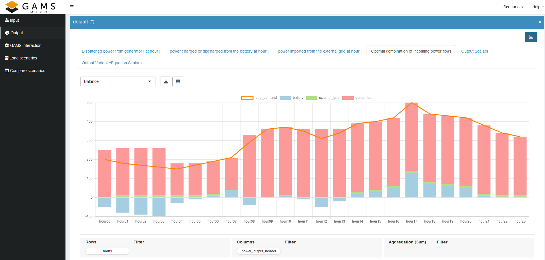
Let’s look at another example. Recall that we combined all power values with the given load demand into a single parameter so we could verify if the load demand is indeed met and how each source contributes at each hour. If we chose a Stacked Bar Chart, we can not easily compare the load demand with the sum of the power sources. Instead, we:

Select Stacked Bar Chart.
Click the icon to add a new view.
In the Combo Chart tab, specify that the load demand should be shown as a Line and excluded from the stacked bars.
Save the view.

The result should look like this:

Here, we can immediately confirm that the load demand is always satisfied - except when the BESS is being charged, which is shown by the negative part of the blue bar. This is another good indication that our constraints are working correctly.

We can create similar visualizations for battery power or external grid power to ensure their constraints are also satisfied. By now, you should have a better grasp of the powerful pivot tool in MIRO and how to use it to check your model implementation on the fly.

Key Takeaways

Interactive Inputs and Outputs: Marking parameters as is_miro_input or is_miro_output enables dynamic fields for data input and real-time feedback, enhancing flexibility and debugging.
Rapid Prototyping: Define output parameters based on variables to summarize important information such as cost. Then visually inspect the output to catch problems early!
Data Validation and Error Reporting: Ensuring input consistency through log files and custom error messages (via MIRO syntax) helps catch errors early and improves user experience by highlighting inconsistencies directly in the input data sheets.
Visual Validation: Pivot tables and charts in MIRO allow you to quickly verify your constraints.
Logical Insights: For example, use stacked bar or line graphs to show whether demand is being met, or which generator combination is the cheapest.

Now that we have our first MIRO application and a better understanding of our optimization model, in the next part we will look at the Configuration Mode, where you can customize your application without writing any code!

GAMS MIRO Walkthrough Part 1