


As artificial intelligence becomes embedded in our phones, computers, and cars, we’re learning that its decision-making can be surprisingly, and worryingly, fragile. In computer vision, for example, nudging the input by adding noise to just a handful of pixels can flip a confident prediction. And what makes it worse is that these systems often feel like black boxes; input goes in, output comes out, and the path in between is hard to see, and harder to evaluate, mainly because the decision process is buried inside millions of learned weights.
That is why evaluating Neural Network’s robustness matters. If small, realistic changes can break a model, we need to know. A practical way to test this is with adversarial attacks; inputs that are intentionally perturbed to push the model towards a wrong decision. While “attacks” sound scary (and can be), they are also a powerful diagnostic tool that allows us to gain evidence in our model’s robustness if it withstands many targeted perturbations. On the other hand, if the model fails, we learn exactly where and how it failed and we try to make it more robust.

Figure 1. Small, targeted pixel changes can swing a model’s prediction, even when the image still looks the same to us.
What’s striking is how subtle these changes are to the human eye. The perturbed digits still read clearly, yet the model’s internal confidence shifts enough to cross a decision boundary. This gap between human perception and model behavior is exactly what we aim to measure and reduce through adversarial robustness testing.
Why does robustness testing matter?
To move from intuition to something we can actually test, using MNIST as our running example, let’s formalize the robustness question that adversarial attacks try to answer:
Given a clean image $x$ with true label $y$, is there a nearby image $x’$ (within a small budget $\varepsilon$) that makes the model prefer some label $\hat{y}\neq y$?
We will call $x’$ “nearby” if, for a chosen norm $\lVert\cdot\rVert$, the distance from $x$ stays within the budget: $$ \lVert x’ - x \rVert \le \varepsilon $$ For images, common choices are the $\ell_\infty$ or $\ell_2$ norms (i.e., $\lVert x’ - x \rVert_\infty \le \varepsilon$ or $\lVert x’ - x \rVert_2 \le \varepsilon$). If no such $x’$ exists, the model is robust to that input at the chosen budget; if one does exist, we’ve found a weak spot.
This approach is valuable because it targets the worst case. Random noise rarely crosses a decision boundary; adversarial noise is crafted precisely to do so. It’s also model-aware: with white-box access we can use gradients or architecture details to search efficiently; with black-box access we can still probe via queries.
What we can’t do is try perturbations by hand. Even a $28\times 28$ MNIST image has $784$ pixels, if you allow each just a few tiny adjustments and the possibilities explode beyond anything we could enumerate. We need a principled way to traverse that space and home in on the most damaging allowed change.
That’s where optimization comes in. In the next section, we’ll turn the question above into a compact mathematical program and show how GAMSPy makes it straightforward to implement and solve—starting with a small MNIST classifier and an objective that directly measures how easily we can push the model off the correct label.
From intuition to an optimization model with GAMSPy
Brute-forcing “tiny pixel nudges” is a non-starter: a single 28×28 image already lives in a 784-dimensional space. Instead, we formulate the attack as an optimization problem and let a solver search that space intelligently.
The idea is simple:
- Start from a correctly classified image $x$.
- Add a bounded perturbation $n$ (our decision variable) with $\lVert n \rVert_\infty \le \epsilon$.
- Pass the perturbed and normalized image through the fixed network.
- Minimize the margin between the score of the correct class and a chosen wrong class:
$$ \min\ y_{right} - y_{wrong}. $$
If the optimum is negative, we found an adversarial example (the wrong class beats the right one). If it’s positive, the model appears robust for that image and budget.
With GAMSPy this is pleasantly direct. Below are the essential pieces from the experiment script we used for this post.
m = gp.Container()
network = build_network(hidden_layers, hidden_layer_neurons)
single_image, single_target = get_image(network)

# 1) Parameters & decision variables
image_data = single_image.numpy().reshape(784)
image = gp.Parameter(m, name="image", domain=dim(image_data.shape), records=image_data)

noise = gp.Variable(m, name="noise", domain=dim([784]))
a1    = gp.Variable(m, name="a1",    domain=dim([784]))

# 2) Bounds: attack budget in pixel space, and valid box after normalization
MNIST_NOISE_BOUND = 0.1     # This is ε, the higher it is, the noisier the image can be
MEAN, STD = (0.1307,), (0.3081,)

noise.lo[...] = -MNIST_NOISE_BOUND
noise.up[...] =  MNIST_NOISE_BOUND
a1.lo[...]    = -MEAN[0] / STD[0]
a1.up[...]    = (1 - MEAN[0]) / STD[0]

# Link normalized input to (image + noise)
set_a1 = gp.Equation(m, "set_a1", domain=dim(a1.shape))
set_a1[...] = a1 == (image + noise - MEAN[0]) / STD[0]

# 3) Embed the trained PyTorch network as equations
seq_formulation = gp.formulations.TorchSequential(m, network)
y, _ = seq_formulation(a1)  # y are the logits/outputs

# 4) Choose the target wrong label = runner-up before perturbation
output_np  = network(single_image.unsqueeze(0)).detach().numpy()[0][0]
right_label = np.argsort(output_np)[-1]
wrong_label = np.argsort(output_np)[-2]

# 5) Objective: minimize the right-vs-wrong margin
obj    = gp.Variable(m, name="z")
margin = gp.Equation(m, "margin")
margin[...] = obj[...] == y[f"{right_label}"] - y[f"{wrong_label}"]

# 6) Solve as a MIP
model = gp.Model(
    m,
    "min_noise",
    equations=m.getEquations(),
    objective=obj,
    sense="min",
    problem="MIP",
)
model.solve(options=gp.Options.fromGams({"reslim": 4000}))
A few notes that make this practical:
-
Network as algebra: TorchSequential lifts a trained PyTorch model into GAMSPy variables and equations, so the solver can reason over the network exactly like any other optimization model.
-
Runner-up target: We set wrong_label to the second highest confidence before adding noise. This often yields a strong, targeted attack with minimal perturbation. Therefore, being robust against this is a good sign.
-
Interpretation: After solving, check one of two outcomes of the objective value: (i) Negative ⇒ attack succeeded (not robust for this image at this budget). (ii) Positive ⇒ the model resisted this attempt.
-
Helper functions: The full code (linked at the end) includes utilities to build the network, load data, and run multiple experiments systematically.
If you would like a slower, step-by-step walkthrough of embedding neural networks and writing these constraints, the GAMSPy Docs have a hands-on tutorial.
ReLU as MIP: exact but combinatorial
ReLU is wonderfully simple in code:
$$\mathrm{ReLU}(s) = \max(0, s).$$
But “max” is piecewise linear, so to represent it exactly in a linear optimization model we usually introduce a binary variable $z$ that says which side of the kink we are on (active or inactive). A standard formulation looks like this (for a neuron with pre-activation $s$ and output $y$):
\begin{aligned} y &\ge s, \quad y \ge 0, \quad \ y &\le s - L(1 - z), \quad\ y &\le Uz, \qquad z \in {0, 1}. \end{aligned}
Here $L$ and $U$ are valid lower/upper bounds on $s$ (the famous “big-M” constants). This is the formulation that most exact robustness verifiers use, and it’s also what you get by default when you embed a PyTorch model with GAMSPy and declare the problem type as MIP, exactly what we did in the code in the previous section:
model = gp.Model(
    m,
    "min_noise",
    equations=m.getEquations(),
    objective=obj,
    sense="min",
    problem="MIP",        # ReLU -> binaries
)
model.solve(solver="cplex")
However, this MIP formulation has some well-known challenges:
-
One binary per ReLU: If your network has $L$ hidden layers with $H$ ReLU neurons each, you already have roughly $L \times H$ binaries (and $\sim 4$ linear constraints) just for the activations. A modest MIP with $3 \times 512$ hidden units means $\sim 1{,}536$ binaries before you’ve modeled anything else.
-
Branch-and-bound combinatorics: MIP solvers explore a tree that branches on these binaries. In the worst case that’s exponential. Good solvers prune aggressively, but as the count grows, so does the search.
In short: the traditional MIP encoding is exact and auditable, but you pay with combinatorial search. For educative models (like the small MNIST MIP we’re using) it works fine; for larger or deeper networks, solve times can skyrocket.
This is precisely why we looked for an alternative. In the next section we’ll swap those binaries for complementarity conditions, turning the problem into a smooth NLP that solves much faster in practice—trading global optimality guarantees for speed.
ReLU via complementarity: an NLP alternative
If binaries are the reason MIPs get heavy, the obvious question is: can we model ReLU without introducing binary variables? Yes, by switching to a complementarity view of the activation and solving the resulting model as a Nonlinear Program (NLP).
ReLU as complementarity
For a neuron with pre-activation $t$ and output $y = \max(0, t)$, we can write
\begin{aligned} y &\ge 0, \quad y - t \ge 0, \quad \ y \cdot (y - t) = 0. \end{aligned}
Where exactly one of $y$ and $y - t$ is positive at the solution, capturing the “on/off” logic without any binary variable. This turns the verification problem from a MIP into an MPCC (a mathematical program with complementarity constraints), which we can tackle efficiently with an NLP solver.
The small changes in code
In GAMSPy, the swap is literally a couple of lines. We tell the TorchSequential wrapper to encode every ReLU with the complementarity formulation and we change the model’s type (NLP) and solver (CONOPT):
def convert_relu(m: gp.Container, layer: torch.nn.ReLU):
    return gp.math.relu_with_complementarity_var

# Tell TorchSequential to use that for all ReLUs
change = {"ReLU": convert_relu}
seq_formulation = gp.formulations.TorchSequential(m, network, change)
y, _ = seq_formulation(a1)

# Same objective as before: minimize the right-vs-wrong margin
obj = gp.Variable(m, name="z")
margin = gp.Equation(m, "margin")
margin[...] = obj[...] == y[f"{right_label}"] - y[f"{wrong_label}"]

# Build an NLP and solve it with CONOPT
model = gp.Model(
    m,
    "min_noise",
    equations=m.getEquations(),
    objective=obj,
    sense="min",
    problem="NLP",
)
model.solve(solver="conopt")
Everything else, the perturbation budget, normalization, runner-up target label, and interpretation of the objective, stays the same as in the MIP code.
The complementarity encoding is built into GAMSPy’s convinience
gp.math.relu_with_complementarity_var()function, so you don’t need to build the equations manually. Additionally, CONOPT plugs in seamlessly viasolver="conopt"which is a robust choice for these NLPs and freely available to GAMSPy Academic users.
How does this help? And what do we give up?
-
Speed: Removing thousands of binaries collapses the branch-and-bound tree into a smooth (though nonconvex) search. In practice, our runs on MNIST-scale MIPs and small CNNs are much faster with the NLP route. We’ll show numbers in the upcoming section.
-
Tradeoff: There is no free lunch! An NLP solver like CONOPT does not guarantee global optimality. You may land on a local minimum with a positive margin even if a negative (successful attack) exists. That’s the price we pay for speed.
This is where strategy matters: if the NLP returns a negative objective, you found a valid adversarial example, period. On the other hand, if it returns a positive objective, we can not be certain the model is robust; we may have just landed in a local minimum. To improve our confidence, we can try multiple starting points of the NLP model (as we will see in section Speed as a strategy).
The trade-off in practice: accuracy vs. speed
Now for the fun part! Here we compare the two formulations head-to-head on a suite of MNIST classifiers, measuring solve time, agreement on the robustness verdict, and false positives (cases where NLP says “robust” but MIP found an attack). The models are ranged from 1 to 5 hidden layers with 10 to 60 neurons each, using a runner-up targeted attack with an $\ell_\infty$ noise budget of $0.1$, keeping the same image, labels, and bounds across both runs.
The two configurations are:
- MIP: ReLU with binaries and
problem="MIP". - NLP: ReLU via complementarity and
problem="NLP"solved with CONOPT. - Both used
reslim = 4000seconds; when the MIP hits that limit, it returns the best bound found so far.
Below, we summarize the three things you probably care about most: speed, agreement on the robustness verdict (sign of the margin), and false positives (cases where NLP says “robust” but MIP found an attack).
Speed
Across the 30 architecture pairs:
- Median solve time: 12.12s for MIP vs 0.227s for NLP.
- Mean solve time: 1004.042s for MIP vs 0.413s for NLP.
- NLP was slower only $1/30$ times (a tiny $0.13\text{s}$ vs $0.16\text{s}$ on the smallest network).
- MIP timeouts: $7/30$ runs hit the $4000\text{s}$ limit (depths $3$–$5$) while all NLP runs finished in under $1.63\text{s}$.
The figure below visualizes the solve times of both methods. Each orange–blue pair corresponds to one architecture (hidden layers × neurons per layer). On the log-scale axis, the vertical gap between each pair is the per-instance speedup: as we move right, networks get wider/deeper, that gap widens dramatically. Even where tiny models are close, MIP escalates by orders of magnitude while the NLP track stays clustered near the bottom axis.
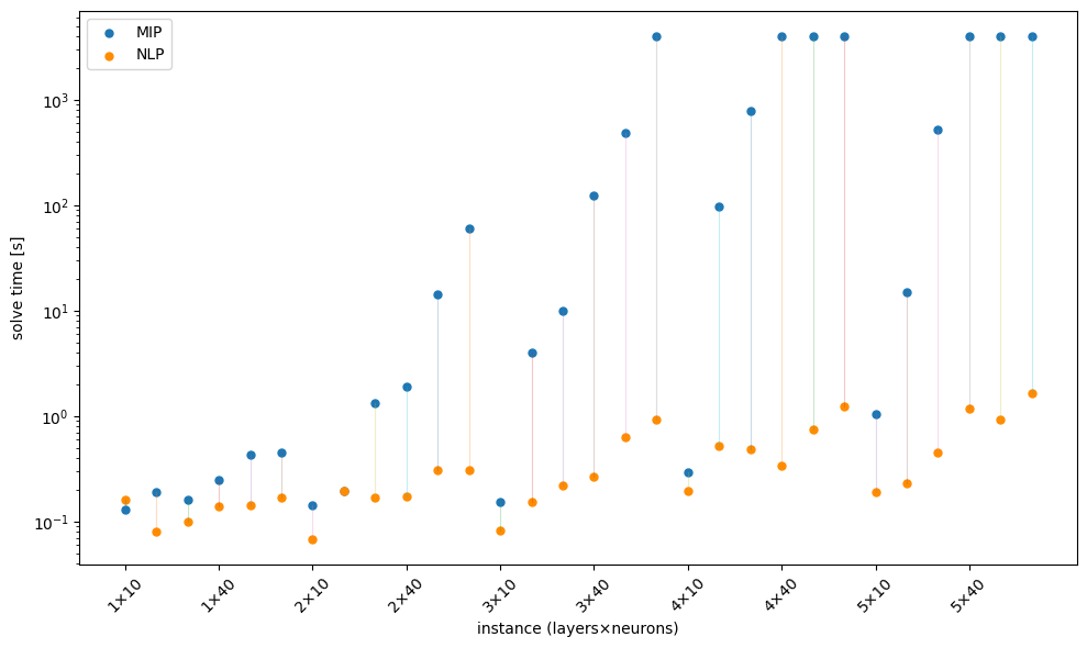
Figure 2. MIP vs NLP solve times per architecture.
Note: the MIP models are also larger on average due to the additional binary variables.
Verdict agreement
We compare the sign of the optimal objective (negative $\Rightarrow$ attack found; positive $\Rightarrow$ “robust” at this budget):
- Exact equality of margins: $12/30$ pairs matched exactly to the $5^{\text{th}}$ decimal place.
- Agreement: $26/30$ pairs agreed on the sign of the margin (both found an attack or both said “robust”).
- Disagreements: $4/30$; in 3 of these, MIP hit the time limit without proving optimality and returned a positive bound, while NLP found a negative margin (successful attack). In the last disagreement, MIP returned a negative margin while NLP returned a positive one (false positive).
False positives
We observed $1/30$ false positive from architecture with $4$ layers and $40$ neurons per layer. Here, MIP found an attack with margin $-1.96$ but NLP returned a positive margin of $+5.49$. This highlights the trade-off: while NLP is fast (This specific run took MIP 4000s, hitting the time limit, while NLP ran for 0.342s), it can miss attacks that MIP finds. To mitigate this, one could run NLP from multiple starting points or use it as a quick filter before applying MIP for confirmation as we discuss next.
Summary table
Below is the detailed results table for all architecture pairs tested for this experiment. As mentioned earlier in the post, the objective function of the study is to minimize margins between the correct and runner-up labels under an $\ell_\infty$ perturbation budget of $0.1$ on a fixed MNIST image. Therefore, negative objective values indicate successful adversarial attacks, while positive values suggest robustness at this budget. What we try to study here is the agreement between MIP and NLP formulations in terms of both objective values and robustness verdicts, along with their respective solve times. Furthermore, the “False Robustness” column flags cases where the NLP formulation incorrectly indicates robustness (positive margin) while the MIP formulation finds an adversarial attack (negative margin). Although there are some cases where the NLP finds stronger attacks (more negative margins) than MIP, those cases are essentially when MIP hits the time limit and returns a suboptimal positive bound (as the MIP solver guarantees global optimality if given enough time).
| Hidden Layers | Neurons / Layer | MIP Objective Value | MIP Solve Time (s) | MIP Variable Count | NLP Objective Value | NLP Solve Time (s) | NLP Variable Count | False Robustness |
|---|---|---|---|---|---|---|---|---|
| 1 | 10 | 3.88899 | 0.130 | 1609 | 5.092 | 0.160 | 1599 | |
| 1 | 20 | 0.49645 | 0.190 | 1639 | 1.04024 | 0.081 | 1619 | |
| 1 | 30 | -0.64841 | 0.160 | 1669 | -0.64841 | 0.099 | 1639 | |
| 1 | 40 | -0.32195 | 0.247 | 1699 | -0.31491 | 0.138 | 1659 | |
| 1 | 50 | -1.35391 | 0.429 | 1729 | -1.16102 | 0.142 | 1679 | |
| 1 | 60 | -1.76911 | 0.455 | 1759 | -1.76911 | 0.170 | 1699 | |
| 2 | 10 | -3.14897 | 0.143 | 1639 | -3.04977 | 0.068 | 1619 | |
| 2 | 20 | 1.95283 | 0.196 | 1699 | 1.95283 | 0.193 | 1659 | |
| 2 | 30 | -1.22023 | 1.319 | 1759 | -1.22023 | 0.168 | 1699 | |
| 2 | 40 | -6.33439 | 1.881 | 1819 | -6.33439 | 0.173 | 1739 | |
| 2 | 50 | -3.47329 | 14.177 | 1879 | -3.47192 | 0.310 | 1779 | |
| 2 | 60 | -6.79947 | 60.539 | 1939 | -6.77727 | 0.311 | 1819 | |
| 3 | 10 | -3.04560 | 0.154 | 1669 | -3.04560 | 0.083 | 1639 | |
| 3 | 20 | -2.28455 | 4.013 | 1759 | -2.28455 | 0.152 | 1699 | |
| 3 | 30 | -0.51342 | 10.063 | 1849 | -0.39979 | 0.221 | 1759 | |
| 3 | 40 | -2.26477 | 123.597 | 1939 | -2.23418 | 0.269 | 1819 | |
| 3 | 50 | -0.81301 | 484.237 | 2029 | -0.80001 | 0.628 | 1879 | |
| 3 | 60 | -6.67975 | 4000.461 | 2119 | -6.63047 | 0.920 | 1939 | |
| 4 | 10 | -9.20940 | 0.295 | 1699 | -9.20940 | 0.194 | 1659 | |
| 4 | 20 | -5.61790 | 96.590 | 1819 | -5.39378 | 0.517 | 1739 | |
| 4 | 30 | -6.18924 | 781.783 | 1939 | -6.18924 | 0.488 | 1819 | |
| 4 | 40 | -1.96277 | 4000.354 | 2059 | 5.48993 | 0.342 | 1899 | Yes |
| 4 | 50 | -7.70052 | 4000.710 | 2179 | -7.70052 | 0.739 | 2019 | |
| 4 | 60 | 7.55647 | 4000.487 | 2299 | -1.81861 | 1.230 | 2059 | |
| 5 | 10 | -5.78419 | 1.038 | 1729 | -5.78419 | 0.190 | 1679 | |
| 5 | 20 | -13.40505 | 15.089 | 1879 | -13.36193 | 0.232 | 1779 | |
| 5 | 30 | -4.55439 | 520.764 | 2029 | -4.55439 | 0.451 | 1879 | |
| 5 | 40 | -1.39833 | 4000.662 | 2179 | -4.98835 | 1.177 | 1979 | |
| 5 | 50 | 14.42331 | 4000.413 | 2329 | -1.78056 | 0.916 | 2079 | |
| 5 | 60 | 5.55635 | 4000.689 | 2479 | -3.79127 | 1.632 | 2179 |
Speed as a strategy
The punchline from the previous section is that the NLP formulation is so much faster than the MIP one, often by orders of magnitude. This speed opens up new strategies to increase our confidence in the robustness verdict, as we afford to run it dozens, hundreds, and even thousands of times. That speed lets us attack the big practical question: If NLP doesn’t guarantee global optimality, how do we raise our confidence that a positive margin isn’t just a local minimum?
One strategy is to run the same NLP model repeatedly from different initial solutions. If any run finds a negative objective, we’ve discovered an adversarial example and can declare the network not robust for that image and budget with certainty. If all runs return positive objectives, we can report that no attack found after N diverse starts, which is a much stronger statement than a single start.
How to initialize multiple NLP runs?
The entire model is driven by the perturbation vector noise. Everything else (normalized input a1, layer outputs, logits y, and the objective) depends on noise via the constraint:
set_a1[...] = a1 == (image + noise - MEAN[0]) / STD[0]
So it’s enough to set an initial level for noise. GAMSPy exposes this as the variable’s level values:
noise_init = <some numpy array of shape (784,)>
noise_vals = gp.Parameter(m, name="noise_vals", domain=noise.domain, records=noise_init)
noise.l[...] = noise_vals[...]   # <-- initial solution
Generating diverse starts with Sobol
Setting noise_init to different values gives different starting points for the NLP solver. And to make use of the speed advantage wisely, we want these starting points to be as diverse as possible within the allowed perturbation box $[-\epsilon, \epsilon]^{784}$. That way, we explore different regions of the search space and reduce the chance of missing an attack. We can achieve this using low-discrepancy sequences, which are designed to fill a space evenly. An excellent choice is the Sobol sequence
and is implemented in scipy.stats.qmc
:
from scipy.stats import qmc

sampler = qmc.Sobol(d=784)
samples = sampler.random_base2(m=10)  # 2^10 = 1024 starts
scaled = qmc.scale(
    samples,
    l_bounds=[-MNIST_NOISE_BOUND]*784,
    u_bounds=[ MNIST_NOISE_BOUND]*784,
)
for sample in scaled:
    build_ad_attack_model(hidden_layers, neurons, mip=False, noise_init=sample)
Early stopping when an attack is found
Since any negative margin proves non-robustness, you can stop the loop as soon as you hit one. We can achieve this by slightly modifying the build_ad_attack_model(...) function in our code to accept an optional noise_init argument and return the objective value after solving. Then, in the loop above, we check the returned margin and break if it’s negative.
for sample in scaled:
    margin_value = build_ad_attack_model(hidden_layers, neurons, mip=False, noise_init=sample)
    if margin_value < 0:
        print("Adversarial example found!")
        break
Revisiting the “false positive”. Can multi-start NLP fix it?
Remember the lone false positive from the previous section (the $4\times 40$ network), where the NLP returned misleading $+5.48993$ margin while the MIP run found $-1.96277$? This is the moment of truth for our multi-start strategy. We can demonstrate its effectiveness by re-running the NLP with Sobol multi-starts and early stopping as described above. The loop stops when the MIP-found attack is rediscovered, this could take just a few or many runs depending on luck and the distribution of local minima. But, here is what happened:
- Run #2 already produced a negative margin $\to$ an actual attack (so the earlier “robust” verdict was just a local minimum).
- Run #5 matched the MIP value $-1.96277$ (within a tight tolerance), showing that the NLP can reach the same minimum when started well.
Takeaway: The “false positive” disappeared as soon as we diversified initializations. notice how MIP took more than an hour to find the attack, while NLP with multi-start found it in under 5 seconds. You still don’t get global guarantees from NLP, but with cheap diversity in starts, you dramatically reduce the chance of a misleading local minimum—while keeping runtimes tiny compared to a full MIP search.
Note: The code shared at the end includes this multi-start strategy with this exact NN for you to try out.
When to escalate to MIP?
The NLP + Sobol multi-start approach is a powerful screening tool, but there are scenarios where you might still want to escalate to the exact MIP formulation for confirmation, such as:
-
If repeated NLP runs only return small positive margins (say $0 < \text{margin} < 1$), or the decision is high-stakes (you need a certificate), switch the exact same model to MIP and let it prove (or disprove) robustness.
-
If the model is small enough that MIP solves quickly (under a minute), you might as well run it directly for a definitive answer.
Otherwise, for screening at scale, NLP + Sobol multi-start is a sweet spot: fast, simple to automate, and per the results of this experiment, usually agrees with globally solved MIPs on the verdict.
Other binary-free ReLU formulations you can try
There isn’t a one-size-fits-all way to encode ReLU for verification. Beyond MIP (big-M + binaries) and the NLP complementarity track you’ve seen, GAMSPy exposes an MPEC route that keeps ReLU’s logic exact without binaries by using equilibrium/complementarity conditions handled by NLPEC solver (Which is also freely available for GAMSPy academic users).
Licensing heads-up: Some users may encounter a license issue when using the NLPEC solver. If this happens, and you’re on an Academic license, please contact us via support@gams.com so we can help resolve access.
Mathematical view
Let $x$ be the pre-activation and $y = \max(0, x)$ the ReLU output. Define the slack
$$ s := y - x. $$
Then ReLU is equivalent to the linear relations plus a single complementarity pair:
$$ y \ge 0 ; \quad s \ge 0 ; \quad s = y - x; \qquad \therefore \quad y \perp s \quad \text{i.e., } y\cdot s = 0 $$
This formulation is an exact representation of ReLU because:
-
If $(x\le 0):$ $(y\ge x)$ and $(y\ge0)$ force $(y=0)$, then $(s=-x\ge0)$.
-
If $(x\ge 0):$ $(y=x\ge0)$ and thus $(s=0)$.
Hence $(\displaystyle y=\max(0,x))$.
Geometrically, the ReLU graph is the union of two polyhedral cones in $(x, y)$: $K_{1} = { x \le 0, y = 0 }$ and $K_{2} = { x \ge 0, y = x }$.
- MIP imposes this disjunction via a binary $z \in {0, 1}$ and big-M inequalities to select either $K_{1}$ or $K_{2}$.
- MPEC enforces mutual exclusivity without a binary: $y \ge 0$, $s \ge 0$, and $y \perp s$ ensure at most one of ${y, s}$ is positive, which picks exactly one cone. No big-M and no branch-and-bound tree.
In optimization terms, each ReLU is a tiny LPCC (linear program with complementarity constraints).
Stacking them yields a network that is an MPCC/MPEC rather than a MIP.
Using the equilibrium-based ReLU in GAMSPy
GAMSPy provides a ready-made generator:
- Function:
gp.math.activation.relu_with_equilibrium - Model type:
problem="MPEC" - Solver:
solver="nlpec"
Drop-in wiring that replaces the ReLU formulation in the earlier code is as follows:
# 1) Swap ReLU layers to the equilibrium-based MPEC encoding
def convert_relu_equilibrium(m: gp.Container, layer: torch.nn.ReLU):
    return gp.math.activation.relu_with_equilibrium

change = {"ReLU": convert_relu_equilibrium}
seq_formulation = gp.formulations.TorchSequential(m, network, change)
y, matches, _ = seq_formulation(a1)

# 2) Objective: same right-vs-wrong margin as before
obj    = gp.Variable(m, name="z")
margin = gp.Equation(m, "margin")
margin[...] = obj[...] == y[f"{right_label}"] - y[f"{wrong_label}"]

# 3) Build an MPEC and solve it with NLPEC
model = gp.Model(
    m,
    "min_noise",
    equations=m.getEquations(),
    objective=obj,
    sense="min",
    problem="MPEC",          # <-- binary-free MPCC/MPEC
    matches=matches,        # <-- complementarity pairs
)
model.solve(solver="nlpec")   # <-- NLPEC handles the equilibrium smoothing
Practical tips
- Keep inputs/activations well-scaled as we have done in the MNIST normalization.
- For robustness screening, combine NLPEC with multi-start initializations of the
noisevector and stop at the first negative margin. - Log NLPEC’s final stationarity/feasibility and the achieved margin for auditability.
Want more MPEC variants?
NLPEC supports several equilibrium/complementarity formulations (e.g., Fischer–Burmeister family and relatives). Some networks/budgets favor one variant over another. You can experiment and benchmark different formulations by swapping out the ReLU generator function in the code above with one of those alternatives you can build yourself. You can find the full list of available complementarity functions in the GAMS NLPEC documentation .
Takeaways & next steps
Along the way, we saw the classic MIP route (exact, certifiable, but slow and impossible to solve as networks grow) and a complementarity-based NLP alternative that delivers the same verdict on most cases in a tiny fraction of the time. That speed is a superpower which can be harnessed to run multiple diverse starts via Sobol sequences, boosting our confidence in the robustness verdict without the combinatorial overhead of MIPs. The output from NLP runs can either find real attacks or provide strong practical evidence of robustness when none emerge. The beauty is in the trade-off; we give up global optimality guarantees for speed, but gain the ability to scale robustness verification to larger models and datasets.
GAMSPy makes it easy to implement both formulations, switch between them, and run experiments at scale with minimal code changes. With just a few lines, you can embed your PyTorch model, set up the adversarial attack optimization, and choose between MIP or NLP formulations, utilizing GAMS powerful solvers under the hood with Python’s simplicity and data-friendly ecosystem.
If you want to dive deeper or adapt the workflow, the GAMSPy docs’ step-by-step tutorial on embedding neural networks is a great place to start; then try this code here . on your network, log your runs, and see where the frontier of robustness really lies.