

Whether you are a modeler at an energy company planning grid transitions, an operations researcher optimizing global supply chains, or a data scientist tackling massive resource allocation problems, your models are likely growing in scope and resolution. The resulting massive linear programs push the shared-memory interior point methods (IPM) that have long been the standard to the limits of their scalability.
GPU-accelerated first-order methods (FOM) have emerged as a serious alternative. In a recent computational study 1, we found that they scale well and deliver short solution times on many instances, especially when a solution of moderate accuracy is good enough.
This post has two goals. First, it shows how easy it is to experiment with GPU-accelerated solvers through GAMS and GAMSPy. Second, it reports on the multi-GPU PDLP solver of NVIDIA cuOpt 26.10: how much faster it gets on 1, 2, 4 and 8 GPUs, which models benefit, and where it still falls short.
Part 1: Experimenting with GPU-accelerated solvers
GAMS gives you access to every practically relevant solver with a GPU-accelerated LP algorithm today:
- NVIDIA cuOpt : a GPU-native optimization engine in which all algorithms run on the GPU.
- Gurobi : the primal-dual hybrid gradient (PDHG) method on the GPU.
- COPT : the first-order PDLP method and the barrier method on the GPU.
- HiGHS : the PDLP and HiPDLP first-order methods on the GPU.
- FICO Xpress : the PDHG method on the GPU.
cuOpt runs on Linux only, and Gurobi’s GPU support is not yet available on Windows. COPT, HiGHS and Xpress also use the GPU on Windows. macOS has no CUDA support at all. Make sure CUDA is installed: nvidia-smi shows the CUDA version your driver supports, and NVIDIA’s CUDA downloads
page has the matching toolkit. The examples below use Linux.
A word on expectations: the speedups reported in Part 2 come from enterprise-grade GPUs, the NVIDIA B200 and H200. Workstation-class hardware, such as the NVIDIA DGX Spark with its GB10 GPU or a desktop PC with a commodity GPU such as an RTX 4000, won’t reach that performance. It does run large LPs, though, and lets you evaluate GPU accelerated methods on your own models. If the results look promising, leasing enterprise GPUs in the cloud is the next step to consider.
1. Install the solvers and their CUDA dependencies
To keep the GAMS distribution small, it doesn’t include cuOpt or the GPU-enabled Gurobi library . Fetching both takes a few commands. After installing GAMS with the standard Linux installer (x86_64 and aarch64 are supported; the example uses aarch64), download the GPU-enabled Gurobi library and the cuOpt helper script into the GAMS system directory. The URL for the Gurobi library is subject to change, so please check the GAMS/Gurobi manual :
mkdir ~/gams && cd ~/gams
curl -O https://d37drm4t2jghv5.cloudfront.net/distributions/latest/linux/linux_arm64_sfx.exe
export DIST=$(curl -s https://www.gams.com/docs/release/distro.txt | head -n 1 | sed -E 's/^\[([0-9]+)([0-9])[0-9],.*/\1.\2/')
chmod u+x linux_arm64_sfx.exe
./linux_arm64_sfx.exe
cd gams${DIST}_linux_arm64_sfx
export PATH=~/gams/gams${DIST}_linux_arm64_sfx:$PATH

# Optional: only needed for Gurobi's GPU PDHG.
curl -O https://d37drm4t2jghv5.cloudfront.net/gurobi/13.0.2/liblax/cuda13/libgurobi.so.13.0.2

curl -O https://raw.githubusercontent.com/GAMS-dev/cuoptlink-builder/main/fetch-cuoptlink.py
python3 fetch-cuoptlink.py install --gams-dir $PWD --cuda-runtime
The script fetch-cuoptlink.py downloads the GAMS/cuOpt link into the GAMS system directory and sets up the CUDA runtime libraries that cuOpt and the other GPU-accelerated solvers need.
With GAMSPy it is even simpler:
pip install gamspy
gamspy install solver copt cuopt gurobi highs xpress

# Optional: only needed for Gurobi's GPU PDHG
cd "$(gamspy show base)"
curl -O https://d37drm4t2jghv5.cloudfront.net/gurobi/13.0.2/liblax/cuda13/libgurobi.so.13.0.2
2. Switch on the GPU methods with solver options
Each solver needs its own options to utilize the GPU:
| Solver | Options | Algorithm on the GPU |
|---|---|---|
| COPT | gpumode=1, lpmethod=6 |
PDLP |
| COPT | gpumode=2, lpmethod=2 |
Barrier |
| cuOpt | none | All algorithms run on the GPU |
| Gurobi | pdhggpu=1, method=6 |
PDHG |
| HiGHS | pdlp_gpu=1, solver="pdlp" or solver="hipdlp" |
PDLP or HiPDLP |
| Xpress | barHGGPU=1, defaultAlg=4, barAlg=4, concurrentThreads=1 |
PDHG |
On the GPU, Xpress runs PDHG in single precision by default, which is faster and needs less memory but limits the accuracy it can reach. For accurate solutions, add barHGPrecision=1 to switch to double precision.
In GAMS, options go into a solver option file
, which the solver reads when the optFile model attribute is set:
model mymodel / all /;

file fopt / highs.opt /;
putclose fopt 'pdlp_gpu=1' / 'solver="hipdlp"' /;
mymodel.optFile = 1;

option solver = highs;
solve mymodel min obj using lp;
In GAMSPy, they are an argument of Model.solve():
import gamspy as gp

m = gp.Container()
...
mymodel = gp.Model(
    m, problem="lp", sense="min", equations=m.getEquations(), objective=obj
)
mymodel.solve(solver="highs", solver_options={"pdlp_gpu": 1, "solver": "hipdlp"})
3. Check the log to confirm the GPU is used
Some solvers quietly fall back to the CPU when the hardware or driver doesn’t meet their requirements. The solver log tells you whether the GPU was used. These are the lines to look for (from runs on an NVIDIA GB10):
| Solver | Log lines confirming the GPU |
|---|---|
| COPT (PDLP) | Hardware has 1 supported GPU device with CUDA 13.0 … Starting PDLP solver using GPU 0 |
| COPT (barrier) | Starting barrier solver using 20 CPU threads and GPU 0 |
| cuOpt | CUDA 13.3, device: NVIDIA GB10 (ID 0), VRAM: 119.63 GiB |
| Gurobi | GPU model: NVIDIA GB10, CUDA compute version 12.1 … Start PDHG on GPU |
| HiGHS | Cuda device 0: NVIDIA GB10 … Using HiPDLP first order PDLP solver on a GPU |
| Xpress | GPU support requested and available, using GPU … CUDA initialized with single precision |
Part 2: Multi-GPU PDLP in NVIDIA cuOpt 26.10
Background
We work closely with Burcin Bozkaya and the cuOpt team at NVIDIA. After our joint work on the MIPFeas benchmark , we turned to large linear programs from energy system modeling, where GAMS customers often face long solution times. Together with GAMS colleagues and researchers at ZIB and DLR (Janina Zittel, Annika Buchholz, Frederik Fiand, Thorsten Koch, Lukas Mehl, Niels Lindner and Manuel Wetzel), we compared shared-memory IPMs, GPU-accelerated FOMs and distributed-memory IPMs on 46 large energy system LPs 1.
NVIDIA then gave us access to an NVIDIA DGX B200 with eight B200 GPUs, on which we evaluated the multi-GPU PDLP (mPDLP) of the released cuOpt 26.10 (git hash: e93f7dc5).
How multi-GPU PDLP splits the work
PDLP spends almost all of its time in sparse matrix-vector products with the constraint matrix and its transpose. mPDLP, introduced in cuOpt 26.08 2, distributes exactly these: it partitions the matrix with a k-way min-cut partitioning of its row-column graph, one part per GPU, so that as few nonzeros as possible connect different GPUs. Presolve, setup, partitioning and postsolve still run once, outside the distributed loop, and communication does not yet overlap with computation 3. The academic D-PDLP solver 4 takes a different route: it splits the matrix into a two-dimensional grid of blocks and balances them with a random block permutation.
NVIDIA reports that the speedup grows with the size of the problem and becomes noticeable above roughly 10 million nonzeros 3. All our instances are larger than that; in our test set, the line falls closer to 25 million nonzeros (see below).
Benchmark setup
- Instances: the 36 of the 46 instances in 1 that at least one method solves within one hour, as reported in 1.
- Hardware: an NVIDIA DGX B200 with eight B200 GPUs and two Intel Xeon Platinum 8570 CPUs.
- cuOpt 26.10: PDLP with PSLP presolve on 1, 2, 4 and 8 GPUs (
num_gpus), with the relative tolerancesrelative_primal_tolerance,relative_dual_toleranceandrelative_gap_toleranceset to 1e-6. - Baselines from 1: the virtual best IPM (VB-IPM) is the fastest of COPT, CPLEX, Gurobi, MOSEK and Xpress barrier on each instance, with 32 threads (also 16 threads) on an Intel Xeon Gold 6342, tolerance 1e-6 and no crossover. The virtual best FOM (VB-FOM) is the fastest of PDHG in Gurobi and Xpress and PDLP in COPT on one NVIDIA H200. cuOpt 26.04 also ran on one H200; some of its times were measured on an H100 and scaled to the H200 1. All first-order methods used tolerance 1e-6 as well.
- Time limit: three hours. Runs that time out, and times above three hours in 1, count as 10,800 seconds.
- Summary measure: the geometric mean of the solution times over all 36 instances, the same instances for every configuration.
All cuOpt logs of these runs on the NVIDIA DGX B200 are available for download
. The share has one folder per configuration, with one log per instance, named <instance>_<folder>.log:
| Folder | Runs |
|---|---|
num-gpus_1, num-gpus_2, num-gpus_4, num-gpus_8 |
1, 2, 4 and 8 GPUs, tolerance 1e-6 |
deftol_num-gpus_8 |
8 GPUs, cuOpt’s default tolerance of 1e-4 |
num-gpus_1_phrm_0 |
1 GPU without column reduction (pdlp_hyper_reduced_matrix=0), for the seven instances where cuOpt applies it (see below) |
Each log starts with the parameter settings, the cuOpt version and the hardware, followed by the problem size before and after presolve, the iteration log, and the final status, objective, iteration count and time.
Results
| Configuration | Hardware | Geometric mean (s) | Timeouts |
|---|---|---|---|
| VB-IPM, 16 threads | Intel Xeon Gold 6342, from 1 | 1,607.2 | 5 |
| VB-IPM, 32 threads | Intel Xeon Gold 6342, from 1 | 1,509.5 | 4 |
| VB-FOM | 1 NVIDIA H200, from 1 | 877.6 | 4 |
| cuOpt 26.04 | 1 NVIDIA H200, from 1 | 592.2 | 4 |
| cuOpt 26.10 | 1 NVIDIA B200 | 631.9 | 5 |
| cuOpt 26.10 | 2 NVIDIA B200 | 484.0 | 4 |
| cuOpt 26.10 | 4 NVIDIA B200 | 380.2 | 4 |
| cuOpt 26.10 | 8 NVIDIA B200 | 355.3 | 5 |
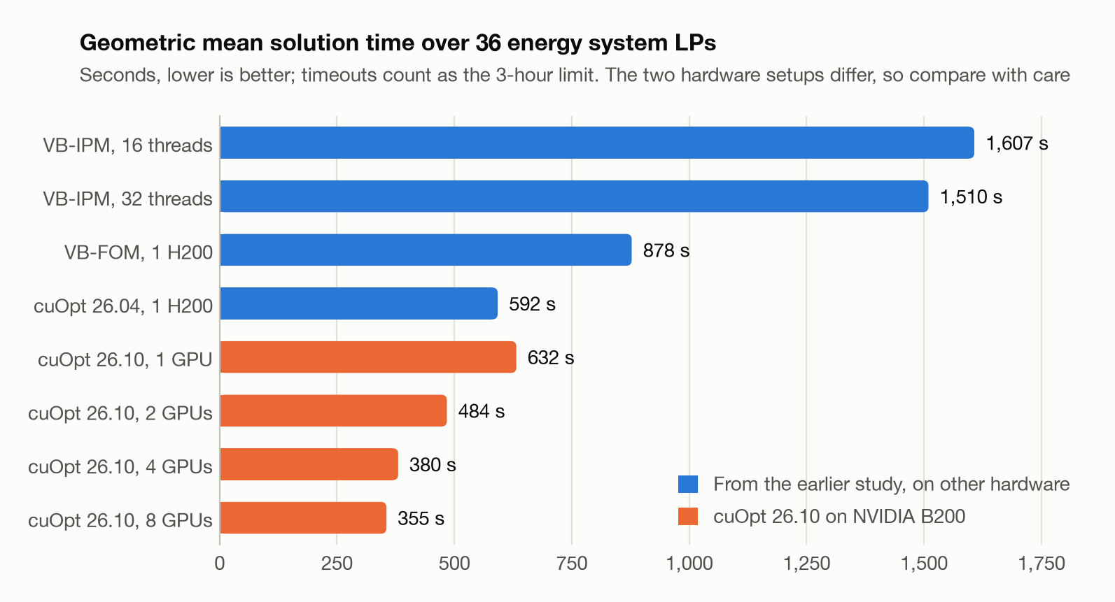
The first four rows come from the study in 1, and are not directly comparable to the DGX B200 runs, given differences in hardware and unstated setup details in the original study. However, because cuOpt was evaluated in both environments, it serves as a common reference point. All geometric means are therefore presented together to illustrate broad performance trends, though precise speedup factors should not be inferred from the chart.
The connecting element holds a surprise: on a single GPU, cuOpt 26.10 on a B200 is slightly slower in geometric mean than cuOpt 26.04 was on an H200 in 1 (631.9 against 592.2 seconds), although the B200 is the newer GPU. The different setups may account for part of that. We have no complete explanation, but we know that PDLP is prone to performance variability: we have seen runs of the same instance take very different numbers of iterations. Interior point methods don’t suffer from variability in this extreme form. Some of their components, such as the ordering algorithm, can have a huge effect on their performance too, but that effect can be observed beforehand and tuned with parameters. Besides mPDLP, cuOpt 26.10 brought other changes to PDLP, such as the new Curtis–Reid scaling, now the default, and column reduction for large problems 2. Changes like these, combined with PDLP’s proneness to variability, can serve as an explanation for the higher geometric mean.
How well does it scale?
To isolate the effect of the GPUs, we ran cuOpt 26.10 on the same server with 1, 2, 4 and 8 GPUs:
| GPUs | Geometric mean (s) | Speedup vs. 1 GPU | Speedup from doubling the GPUs |
|---|---|---|---|
| 1 | 631.9 | 1.00x | |
| 2 | 484.0 | 1.31x | 1.31x |
| 4 | 380.2 | 1.66x | 1.27x |
| 8 | 355.3 | 1.78x | 1.07x |
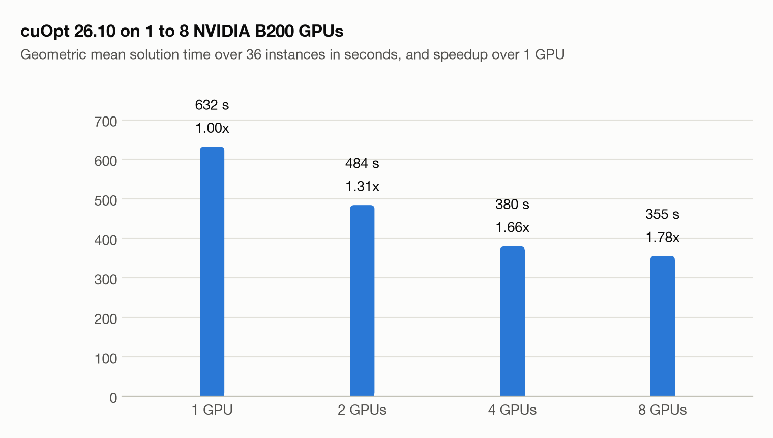
Eight GPUs make cuOpt 1.78 times faster than one, and most of that gain comes from the first two doublings: going from four to eight GPUs adds only 7%. These numbers use cuOpt’s PDLP default settings (other than for tolerances), under which one GPU reduces the columns of some large problems but several GPUs don’t (more on this below). With that reduction switched off, one GPU needs 656.2 seconds in geometric mean, and eight GPUs are 1.85 times faster. Doubling the CPU threads of the IPMs from 16 to 32 helps even less, 6%, so neither kind of hardware turns more parallelism into proportionally shorter solution times. At eight GPUs, the hardware cost per unit of speedup is high, and for most users one or two GPUs will be the sensible choice today.
Which models benefit?
To compare like with like, this section uses the one-GPU runs without column reduction, so that one GPU and eight GPUs run the same algorithm.
The geometric mean hides a wide spread. Of the 31 problems solved by both configurations, 19 ran at least twice as fast on eight GPUs, with a maximum speedup of 3.94x (BEAM_2016_11_8). However, seven instances gained less than 20%, and one (pypsa-de-elec-50-1h) was even slightly slower. In six cases, four GPUs performed better than eight. Five benchmark instances timed out on both configurations.
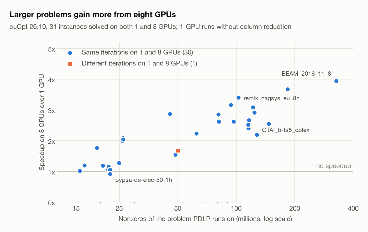
On 30 of these 31 instances, cuOpt takes exactly the same number of iterations on one and eight GPUs. There, the speedup measures the hardware alone, and it follows the size of the problem PDLP works on: the rank correlation between the nonzeros after presolve and the 8-GPU speedup is 0.82. The nine instances with fewer than 25 million nonzeros gain 1.16x in geometric mean, and all but nt2030_2030_CY2009_st1 (1.77x) less than 1.3x. The 21 larger ones gain between 1.55x and 3.94x, 2.62x in geometric mean. What counts is the number of nonzeros, not the number of rows: after presolve, industrial_02 to industrial_04 have fewer than a million rows but 115 million nonzeros, and they run about 2.5 times faster on eight GPUs.
Two effects hold the smaller models back. Each GPU gets too little work per iteration to make up for the communication between the GPUs. And everything before the first PDLP iteration, from presolve to partitioning, runs once and takes the same time on any number of GPUs. On genx-elec_co2-15-168h, for example, that part takes 218 of the 345 seconds on eight GPUs.
Now to the column reduction. On one GPU, cuOpt 26.10 reduces the columns of seven of these large problems before solving them; on several GPUs, it doesn’t. With column reduction, the seven take a different number of iterations on one GPU than on several, so the comparison of one GPU with eight would also compare two slightly different algorithms. I therefore reran them on one GPU with column reduction switched off (pdlp_hyper_reduced_matrix=0), and they then take exactly the same number of iterations as on two to eight GPUs. Column reduction does pay off on a single GPU, though: without it, one GPU is slower on six of the seven, by up to 1.69 times (industrial_05), and faster only on OTAI_b-ts5_cplex (672 instead of 1,459 seconds). Only industrial_14 takes a slightly different number of iterations on eight GPUs than on one.
Accuracy against speed
cuOpt stops when three conditions hold at the same time 5: the primal infeasibility is at most absolute_primal_tolerance + relative_primal_tolerance · ‖b‖₂, the dual infeasibility is at most absolute_dual_tolerance + relative_dual_tolerance · ‖c‖₂, and the duality gap is at most absolute_gap_tolerance + relative_gap_tolerance · (|primal objective| + |dual objective|). The log reports the relative values at the end. For 288_22_8 on eight GPUs, for example, the relative duality gap is 9.8e-7, the relative primal infeasibility 2.9e-8 and the relative dual infeasibility 2.1e-7, all within 1e-6. Because the infeasibilities are measured relative to the norms of the right-hand side (b) and the objective (c), the same tolerance can allow quite different absolute violations on different models. Moreover, cuOpt applies these criteria to the scaled model; after unscaling, even the relative criteria can be violated.
All results above use relative tolerances of 1e-6. With cuOpt’s PDLP default tolerances of 1e-4, eight GPUs need only 130.2 seconds in geometric mean, 2.73 times less than at 1e-6, and solve 34 instead of 31 instances within three hours. On most instances, the objective value differs by less than 0.1% from the 1e-6 run. Whether the lower accuracy is good enough depends on the application.
Where it falls short
First-order methods are not yet a replacement for interior point methods on every model. Five instances that the IPMs solve within three hours (four of them actually even within one hour) time out with cuOpt 26.10 on eight GPUs. JRC-EU-TIMES-dispatch-30-2016ts is on the brink of infeasibility: how the tolerances are interpreted decides whether it is feasible. cuOpt’s presolve PSLP declares it infeasible, while the other solvers don’t. Because of the problem’s large coefficient range, cuOpt doesn’t trust that verdict and runs PDLP on the original unpresolved problem instead, where it diverges. Reliability across a whole model family matters as much as speed on average. We’re in close contact with the NVIDIA team about these cases.
Final thoughts and an invitation
What I value about GAMS is that it is more than one software stack for many solvers. GAMS is also a solver license broker, so a single point of contact gives you access to all relevant solvers, commercial and open source alike. You can try them on your model and run them on modern hardware, from distributed compute clusters to state-of-the-art GPUs, without changing the model or setup. The speedups shown here need high-end GPUs. Smaller hardware such as a DGX Spark or a workstation GPU won’t match them, but it is a good place to find out whether first-order methods suit your models before you lease enterprise hardware in the cloud.
Today, the main bottleneck is access to that hardware. On Amazon EC2, for example, high-end GPU instances often require a capacity reservation rather than spot instances. We expect this to ease as GPU capacity grows across cloud platforms.
In the meantime, our collaboration with NVIDIA lets us help customers evaluate GPU-accelerated methods on their own models on high-end hardware. Together, we’ll find the setup that fits each case.
The fastest solver is rarely the whole answer, though. Reliability across your model classes, diagnostics such as infeasibility detection, and licensing cost matter just as much. With our broad solver portfolio, a flexible platform, and decades of experience in algebraic modeling and optimization, GAMS can give you neutral, data-driven advice for your requirements.
If you would like to test your models on high-end GPU hardware, or find the solver setup that best fits your technical and financial needs, check out our Solver Evaluation Service and contact us at evaluation@gams.com .
Appendix: solution times per instance
Solution times in seconds; timeouts are runs that did not finish within three hours. VB-IPM uses 32 threads; cuOpt 26.10 runs on B200 GPUs. The runs without column reduction exist only for the instances where cuOpt applies it on one GPU (– for the others).
| Instance | VB-IPM | VB-FOM | cuOpt 26.04 | cuOpt 26.10, 1 GPU | 1 GPU, no column reduction | 2 GPUs | 4 GPUs | 8 GPUs |
|---|---|---|---|---|---|---|---|---|
| 288_22_8 | 3,327 | 425 | 229 | 428 | 679 | 424 | 299 | 259 |
| 672_22_8_cli | timeout | 1,530 | 204 | 973 | 1,365 | 766 | 489 | 372 |
| BEAM_2016_11_8 | timeout | 2,451 | 1,385 | 2,055 | 2,444 | 1,370 | 802 | 620 |
| genx-elec_co2-15-168h | 931 | 778 | 1,021 | 370 | – | 361 | 355 | 345 |
| genx-elec_trex-15-168h | 986 | 670 | 609 | 124 | – | 120 | 113 | 108 |
| genx-elec_trex_co2-15-168h | 1,139 | 401 | 522 | 428 | – | 414 | 456 | 405 |
| industrial_01 | 1,528 | 690 | 403 | 310 | – | 187 | 136 | 108 |
| industrial_02 | 543 | 296 | 62 | 156 | – | 103 | 80 | 65 |
| industrial_03 | 571 | 305 | 68 | 237 | – | 152 | 109 | 89 |
| industrial_04 | 556 | 267 | 48 | 219 | – | 141 | 101 | 87 |
| industrial_05 | 584 | 984 | 628 | 259 | 437 | 264 | 183 | 150 |
| industrial_06 | 592 | 843 | 513 | 368 | 617 | 370 | 252 | 200 |
| industrial_07 | 518 | 406 | 311 | 336 | 379 | 233 | 163 | 130 |
| industrial_08 | 368 | 217 | 45 | 147 | – | 99 | 78 | 74 |
| industrial_09 | 400 | 226 | 56 | 142 | – | 96 | 77 | 68 |
| industrial_10 | 424 | 287 | 65 | 151 | – | 102 | 75 | 74 |
| industrial_12 | 3,440 | 5,626 | 6,162 | timeout | – | timeout | timeout | timeout |
| industrial_13 | 1,475 | 540 | 172 | 99 | – | 77 | 63 | 64 |
| industrial_14 | 3,671 | 9,489 | 3,278 | 6,155 | – | 4,995 | 3,916 | 3,671 |
| JRC-EU-TIMES-dispatch-30-2016ts | 571 | 355 | timeout | timeout | – | timeout | timeout | timeout |
| nt2030_2030_CY2009_st1 | 482 | 505 | 385 | 430 | – | 310 | 243 | 243 |
| oemofB3_int_37 | 3,061 | timeout | timeout | timeout | – | timeout | timeout | timeout |
| OTAI_b-ts5_cplex | 2,950 | timeout | 4,006 | 1,459 | 672 | 425 | 312 | 306 |
| pypsa-de-elec-50-1h | 911 | 188 | 147 | 22 | – | 24 | 21 | 24 |
| pypsa-de-sec-20-1h | 3,415 | timeout | 7,288 | 8,373 | – | 5,390 | 3,866 | 3,744 |
| pypsa-eur-elec-100-3h | 686 | 1,015 | 154 | 367 | – | 290 | 258 | 308 |
| remix_nagsys_cwe_3h | 7,274 | 3,386 | 2,601 | 8,424 | – | 4,953 | 3,386 | 3,215 |
| remix_nagsys_eu_8h | timeout | 2,398 | 1,906 | 4,984 | – | 2,946 | 1,741 | 1,465 |
| remix_nagsys_fr_1h | 4,484 | 7,497 | 2,704 | timeout | – | timeout | timeout | timeout |
| remix_unseen_adalpert_1h | timeout | 854 | 1,229 | 2,147 | – | 1,405 | 992 | 843 |
| remix_unseen_gunilpert_1h | 9,399 | 743 | 590 | 408 | – | 255 | 173 | 143 |
| remix_yssp_disp_488r_1h | 3,698 | 665 | timeout | 519 | – | 319 | 206 | 164 |
| spineopt-multiyear-invest-eu-case-study | 2,352 | timeout | timeout | timeout | – | 9,670 | 8,419 | timeout |
| SWITCH-China-open-model-32-433ts | 112 | 20 | 129 | 73 | – | 71 | 62 | 72 |
| TIMES-GEO-global-base-31-20ts | 759 | 57 | 88 | 51 | – | 42 | 36 | 40 |
| TIMES-GEO-global-netzero-31-20ts | 879 | 880 | 173 | 58 | – | 50 | 42 | 49 |
Appendix: problem size and iterations per instance
Nonzeros of the problem PDLP ran on, in millions (after presolve; for JRC-EU-TIMES-dispatch-30-2016ts, cuOpt distrusted presolve’s verdict of infeasibility and ran on the original problem). Iterations of cuOpt 26.04 as reported in 1 (– for JRC-EU-TIMES-dispatch-30-2016ts, which it declared infeasible), and of cuOpt 26.10 at tolerance 1e-6 and at the default tolerance of 1e-4 on eight GPUs. Runs that hit the time limit show the iterations done until then.
| Instance | Nonzeros solved (M) | cuOpt 26.04 | cuOpt 26.10, 1 GPU | 1 GPU, no column reduction | 2 GPUs | 4 GPUs | 8 GPUs | 8 GPUs, tolerance 1e-4 |
|---|---|---|---|---|---|---|---|---|
| 288_22_8 | 81.3 | 142,000 | 458,200 | 751,200 | 751,200 | 751,200 | 751,200 | 88,400 |
| 672_22_8_cli | 183.8 | 52,800 | 463,200 | 670,800 | 670,800 | 670,800 | 670,800 | 133,000 |
| BEAM_2016_11_8 | 327.6 | 220,600 | 536,400 | 655,600 | 655,600 | 655,600 | 655,600 | 191,800 |
| genx-elec_co2-15-168h | 21.8 | 1,617,400 | 499,600 | – | 499,600 | 499,600 | 499,600 | 86,800 |
| genx-elec_trex-15-168h | 22.0 | 1,015,600 | 362,400 | – | 362,400 | 362,400 | 362,400 | 75,600 |
| genx-elec_trex_co2-15-168h | 22.4 | 747,200 | 682,800 | – | 682,800 | 682,800 | 682,800 | 91,400 |
| industrial_01 | 45.6 | 262,800 | 313,400 | – | 313,400 | 313,400 | 313,400 | 77,400 |
| industrial_02 | 115.5 | 49,000 | 182,200 | – | 182,200 | 182,200 | 182,200 | 42,800 |
| industrial_03 | 116.3 | 54,200 | 292,200 | – | 292,200 | 292,200 | 292,200 | 43,400 |
| industrial_04 | 115.3 | 36,200 | 269,200 | – | 269,200 | 269,200 | 269,200 | 37,000 |
| industrial_05 | 123.8 | 529,000 | 502,200 | 522,600 | 522,600 | 522,600 | 522,600 | 79,400 |
| industrial_06 | 122.1 | 439,200 | 677,000 | 761,800 | 761,800 | 761,800 | 761,800 | 58,800 |
| industrial_07 | 124.1 | 257,200 | 439,200 | 450,200 | 450,200 | 450,200 | 450,200 | 38,000 |
| industrial_08 | 25.9 | 37,600 | 271,400 | – | 271,400 | 271,400 | 271,400 | 35,800 |
| industrial_09 | 26.1 | 51,400 | 261,000 | – | 261,000 | 261,000 | 261,000 | 35,600 |
| industrial_10 | 26.2 | 60,800 | 280,200 | – | 280,200 | 280,200 | 280,200 | 23,800 |
| industrial_12 | 54.9 | 3,822,600 | 12,921,600 | – | 14,481,800 | 20,957,000 | 27,370,200 | 25,905,400 |
| industrial_13 | 48.7 | 117,600 | 85,800 | – | 85,800 | 85,800 | 85,800 | 20,600 |
| industrial_14 | 50.2 | 2,162,600 | 7,914,000 | – | 7,914,000 | 7,914,000 | 8,031,600 | 6,765,600 |
| JRC-EU-TIMES-dispatch-30-2016ts | 369.7 | – | 4,139,200 | – | 7,482,600 | 12,979,200 | 18,329,200 | 17,506,200 |
| nt2030_2030_CY2009_st1 | 19.2 | 502,800 | 996,600 | – | 998,600 | 996,600 | 996,600 | 78,400 |
| oemofB3_int_37 | 69.7 | 12,318,400 | 9,463,800 | – | 14,570,600 | 17,918,200 | 20,892,000 | 2,671,200 |
| OTAI_b-ts5_cplex | 127.5 | 1,432,600 | 585,200 | 421,200 | 421,200 | 421,200 | 421,200 | 76,400 |
| pypsa-de-elec-50-1h | 22.4 | 194,200 | 26,800 | – | 26,800 | 26,800 | 26,800 | 11,200 |
| pypsa-de-sec-20-1h | 62.3 | 3,195,600 | 7,563,800 | – | 7,563,800 | 7,563,800 | 7,563,800 | 745,000 |
| pypsa-eur-elec-100-3h | 16.6 | 267,400 | 1,176,800 | – | 1,176,800 | 1,176,800 | 1,176,800 | 186,400 |
| remix_nagsys_cwe_3h | 96.9 | 1,082,400 | 5,130,000 | – | 5,130,000 | 5,130,000 | 5,130,000 | 1,519,000 |
| remix_nagsys_eu_8h | 102.6 | 744,600 | 2,844,800 | – | 2,844,800 | 2,844,800 | 2,844,800 | 763,200 |
| remix_nagsys_fr_1h | 66.7 | 1,563,600 | 9,237,000 | – | 13,818,200 | 21,434,400 | 19,462,000 | 1,399,800 |
| remix_unseen_adalpert_1h | 147.0 | 209,000 | 581,400 | – | 581,400 | 581,400 | 581,400 | 25,000 |
| remix_unseen_gunilpert_1h | 81.0 | 244,600 | 234,800 | – | 234,800 | 234,800 | 234,800 | 6,700 |
| remix_yssp_disp_488r_1h | 93.6 | 19,029,000 | 272,800 | – | 272,800 | 272,800 | 272,800 | 96,000 |
| spineopt-multiyear-invest-eu-case-study | 20.3 | 22,792,400 | 36,292,200 | – | 39,519,400 | 39,843,000 | 42,177,000 | 3,575,600 |
| SWITCH-China-open-model-32-433ts | 15.6 | 236,400 | 246,600 | – | 246,600 | 246,600 | 246,600 | 15,000 |
| TIMES-GEO-global-base-31-20ts | 24.9 | 154,200 | 151,000 | – | 151,000 | 151,000 | 151,000 | 76,800 |
| TIMES-GEO-global-netzero-31-20ts | 20.6 | 376,400 | 211,200 | – | 211,200 | 211,200 | 211,200 | 78,000 |
References
-
J. Zittel, A. Buchholz, M. Bussieck, F. Fiand, T. Koch, L. Mehl, N. Lindner, M. Wetzel: Computational acceleration strategies for large-scale energy system optimization: a comparative study of GPU-accelerated and distributed-memory solvers . arXiv:2605.04605, 2026. ↩︎ ↩︎ ↩︎ ↩︎ ↩︎ ↩︎ ↩︎ ↩︎ ↩︎ ↩︎ ↩︎ ↩︎ ↩︎ ↩︎
-
NVIDIA: cuOpt 26.10 release notes . ↩︎ ↩︎
-
NVIDIA: Scaling decision optimization to 100 million variables and beyond with mPDLP in NVIDIA cuOpt . ↩︎ ↩︎
-
H. Li, Y. Huang, H. Liu, D. Ge, Y. Ye: D-PDLP: Scaling PDLP to distributed multi-GPU systems . arXiv:2601.07628, 2026. ↩︎
-
NVIDIA: cuOpt LP and MILP settings . ↩︎