Table of Contents
Once a model is completed, it is almost always used to investigate alternative scenarios where the analyst compares the results of various scenario assumptions. In this tutorial we will show how such comparative analyses (also called sensitivity analyses) are done with GAMS. We will first demonstrate an easy approach, where we will manually change input parameters, use repeated solves and generate reports. In a second step, we will introduce another approach, where a loop structure will be used to automatically cycle through the scenarios. We recommend to read the sections on the manual approach first, since the sections on the automated approach build on code blocks developed in the early sections.
Manual Approach
Suppose we wish to do a comparative analysis by altering some input data in a model. We will use as an example the farm profit-maximizing model farmcomp.gms. The following vector of prices for primary commodities is a part of the input data:
Parameter price(primary)  'prices for products in USD'
         / corn  2.20, soybeans   5.00, beef   0.50 /;
We will use these data as a base case and compare it with two alternative scenarios: in the first scenario we will change the price of beef to $0.70 and in the second scenario we will change the price of corn to $2.70.
The GAMS file farmrep.gms is related to our example model. It contains only calculations for report writing and may be included with the dollar control option $include. It will generate a report based on the solution of the last solve that was executed in the GAMS program farmcomp.gms. The report consists of several tables. We will focus on the table Farm Summary that is associated with the parameter summary. The relevant code is given below:
Set  alli 'allitems'
        / corn, soybeans, beef, cattle,
          water, cropland, pastureland,
          fertilizer, seed, othercost, veterinary, supplement,
          "April labor", "May labor", "summer labor", "Sept labor", "Oct labor",
          cattlefeed, total / ;

Set  measures 'output measures'
        / "Net Income",  "Land Use", "Dry Cropping", "Irr Cropping",
          "Livestock", "Resource Value", "Product Value" /

Parameter summary(alli,measures)   'Farm Summary';
Note that the table for the parameter summary will contain rows for the commodities which are elements of the set alli and columns for all elements of the set measures.
We will use a third GAMS file, mancomp.gms,for our comparative analysis. The code of this third GAMS file follows:
$include farmcomp.gms
display price;
$include farmrep.gms

price("beef") = 0.70;
solve farm using LP maximizing netincome;
display price;
$include farmrep.gms

price("corn") = 2.70;
solve farm using LP maximizing netincome;
display price;
$include farmrep.gms
Note that this code first solves the original model that also contains the set definitions for the report, displays the initial prices and generates a report. In a second step the price for beef is changed to $0.70, the modified model is solved, the prices for the first alternative scenario are displayed and a report is generated. In a third step the price for corn is changed to $2.70, the model is solved again, the prices for the second alternative scenario are displayed and a third report is generated. Note that in the second alternative scenario (the third solve) the beef price is $0.70, since it was not reset to base levels after the second run.
There will be three tables associated with the parameter summary in the listing file, one for each solve. The first table reports the results associated with the base case:
----    279 PARAMETER summary  Farm Summary

             Net Income    Land use  Dry Cropp~  Irr Cropp~   Livestock  Resource ~  Product V~

Corn                                      20.00      200.00                                2.20
Soybeans                                 480.00                                            5.00
Beef                                                                                       0.50
cattle                                                           615.79
Water                                                                         16.83
Cropland                     700.00                                          128.49
Pastureland                  130.00                                           84.26
April Labor                                                                   32.34
May Labor                                                                     27.01
Oct Labor                                                                     11.50
Cattlefeed                                                                                 4.71
Total         162685.05                  500.00      200.00
The second table reports the results from the first alternative scenario where the price for beef was changed to $0.70:
----    351 PARAMETER summary  Farm Summary

             Net Income    Land use  Dry Cropp~  Irr Cropp~   Livestock  Resource ~  Product V~

Corn                                      22.84      160.85                                2.34
Soybeans                                 489.86                                            5.00
Beef                                                                                       0.70
cattle                                                           866.67
Cropland                     673.55
Pastureland                  130.00                                         1456.90
April Labor                                                                   82.29
May Labor                                                                     80.53
Sept Labor                                                                    53.57
Oct Labor                                                                     46.21
Cattlefeed                                                                                 4.89
Total         373686.10                  512.70      160.85
And the third table reports the results from the second alternative scenario where the price for corn was changed to $2.70 and the price for beef stayed at $0.70:
----    423 PARAMETER summary  Farm Summary

             Net Income    Land use  Dry Cropp~  Irr Cropp~   Livestock  Resource ~  Product V~

Corn                                      31.98      200.00                                2.70
Soybeans                                 410.24                                            5.00
Beef                                                                                       0.70
cattle                                                           866.67
Water                                                                         15.99
Cropland                     642.22
Pastureland                  130.00                                         1316.09
April Labor                                                                   61.39
May Labor                                                                     61.72
Sept Labor                                                                    84.92
Oct Labor                                                                     87.21
Cattlefeed                                                                                 5.36
Total         375839.30                  442.22      200.00
This quick way to do a comparative analysis has the following drawbacks:
- The relevant output is spread over more than 140 lines.
- There is no cross-scenario report.
- The price of beef in the second alternative scenario is problematic, since it was not automatically reset to the original base price.
- The handling of solves and report writing is repetitive.
The first two issues will be addressed in section Writing Cross-Scenario Reports,a solution for the third issue will be given in section Resetting Data to Base Levels and an alternative approach that will resolve the last issue is presented in section An Automated Approach - Avoiding Repeated Work.
Writing Cross-Scenario Reports
We will generate a cross-scenario report by introducing two new sets and a new parameter in a revised version of the third GAMS file, mancompb.gms:
Set scenarios / base, beefp, beefcorn /;
Set ordr      / "Scenario Setup", "Scenario Results"/;

Parameter savsumm(ordr,*,alli,scenarios)  'Comparative Farm Summary';
savsumm("Scenario Setup","price",primary,"base") = price(primary);
savsumm("Scenario Results",measures,alli,"base") = summary(alli,measures);
Note that the set scenarios contains the base case and the two alternative scenarios and the set ordr introduces places to save the assumptions and results of the different runs. The new parameter savsumm is similar to the parameter summary introduced above, but it has two additional dimensions. Observe that the first assignment copies the current setup of the price vector and the second assignment copies the results that are stored in the parameter summary.
The full code follows:
$include farmcomp.gms
$include farmrep.gms
Set ordr / "Scenario Setup", "Scenario Results" /;
Set scenarios / base, beefp, beefcorn /;
Parameter savsumm(ordr,*,alli,scenarios)  'Comparative Farm Summary';
savsumm("Scenario Setup","price",primary,"base") = price(primary);
savsumm("Scenario Results",measures,alli,"base") = summary(alli,measures);

price("beef") = 0.70;
solve farm using LP maximizing netincome;
display price ;
$include farmrep.gms
savsumm("Scenario Setup","price",primary,"beefp") = price(primary);
savsumm("Scenario Results",measures,alli,"beefp") = summary(alli,measures);

price("corn") = 2.70;
display price ;
solve farm using LP maximizing netincome;
$include Farmrep.gms
savsumm("Scenario setup","price",primary,"beefcorn") = price(primary);
savsumm("Scenario Results",measures,alli,"beefcorn") = summary(alli,measures);

option savsumm:2:3:1;
display savsumm;
Observe that the last index in the assignments for savsumm is "base" after the first solve, "beefp" after the second solve and "beefcorn" after the third solve. Note that option statement in the penultimate line of the code customizes the output generated by the display statement that follows. For details see section Local Display Control. The listing file will contain the following output:
----    436 PARAMETER savsumm  Comparative Farm Summary

                                                   base       beefp    beefcorn

Scenario Setup  .price         .Corn               2.20        2.20        2.70
Scenario Setup  .price         .Soybeans           5.00        5.00        5.00
Scenario Setup  .price         .Beef               0.50        0.70        0.70
Scenario Results.Net Income    .Total         162685.05   373686.10   375839.30
Scenario Results.Land use      .Cropland         700.00      673.55      642.22
Scenario Results.Land use      .Pastureland      130.00      130.00      130.00
Scenario Results.Dry Cropping  .Corn              20.00       22.84       31.98
Scenario Results.Dry Cropping  .Soybeans         480.00      489.86      410.24
Scenario Results.Dry Cropping  .Total            500.00      512.70      442.22
Scenario Results.Irr Cropping  .Corn             200.00      160.85      200.00
Scenario Results.Irr Cropping  .Total            200.00      160.85      200.00
Scenario Results.Livestock     .cattle           615.79      866.67      866.67
Scenario Results.Resource Value.Water             16.83                   15.99
Scenario Results.Resource Value.Cropland         128.49
Scenario Results.Resource Value.Pastureland       84.26     1456.90     1316.09
Scenario Results.Resource Value.April Labor       32.34       82.29       61.39
Scenario Results.Resource Value.May Labor         27.01       80.53       61.72
Scenario Results.Resource Value.Sept Labor                    53.57       84.92
Scenario Results.Resource Value.Oct Labor         11.50       46.21       87.21
Scenario Results.Product Value .Corn               2.20        2.34        2.70
Scenario Results.Product Value .Soybeans           5.00        5.00        5.00
Scenario Results.Product Value .Beef               0.50        0.70        0.70
Scenario Results.Product Value .Cattlefeed         4.71        4.89        5.36
In this cross-scenario report all output is in one table and it is easy to compare the base case with the two alternative scenarios.
We could also add percentage change calculations by introducing a further parameter, savsummp:
Parameter savsummp(ordr,*,alli,scenarios) 'Comparative Farm Summary (percent chg)';

savsummp(ordr,measures,alli,scenarios)$savsumm(ordr,measures,alli,"base") =
   round{ [savsumm(ordr,measures,alli,scenarios) - savsumm(ordr,measures,alli,"base")]*100
   / savsumm(ordr,measures,alli,"base"),1 };

savsummp(ordr,measures,alli,scenarios)
   $[(savsumm(ordr,measures,alli,"base") = 0) and (savsumm(ordr,measures,alli,scenarios) <> 0)]
   = na;

option savsummp:1:3:1;
display savsummp;
Note that both assignment statements are conditional assignments. The first assignment computes percentage changes rounded to one decimal place and the second assignment sets the percentage change to NA if the value in the base case is zero. The output generated by the display statement follows:
----    450 PARAMETER savsummp  Comparative Farm Summary (percent chg)

                                                  beefp    beefcorn

Scenario Results.Irr Cropping  .Corn              -19.6
Scenario Results.Irr Cropping  .Total             -19.6
Scenario Results.Livestock     .cattle             40.7        40.7
Scenario Results.Resource Value.Water            -100.0        -5.0
Scenario Results.Resource Value.Cropland         -100.0      -100.0
Scenario Results.Resource Value.Pastureland      1629.0      1461.9
Scenario Results.Resource Value.April Labor       154.4        89.8
Scenario Results.Resource Value.May Labor         198.1       128.5
Scenario Results.Resource Value.Sept Labor           NA          NA
Scenario Results.Resource Value.Oct Labor         301.8       658.4
Scenario Results.Product Value .Corn                6.4        22.7
Scenario Results.Product Value .Beef               40.0        40.0
Scenario Results.Product Value .Cattlefeed          3.9        13.8
Resetting Data to Base Levels
In the example above the price for beef was changed to $0.70 for the first alternative scenario and it stayed at $0.70 in the second alternative scenario, since we did not reset it manually to the base level. However, in most cases users find it preferable to reset all data to base levels before a new scenario is run. This may be done by saving the base level data in a new parameter, say saveprice, and then resetting the data to base levels before each scenario. In the following final version of the third GAMS file, mancompc.gms, the levels of the commodity prices are reset before each new run:
$include farmcomp.gms
$include farmrep.gms

Parameter saveprice(alli) 'saved prices';
saveprice(alli) = price(alli);

Set scenarios / base, beefp, beefcorn /;
Parameter savsumm(ordr,*,alli,scenarios)  'Comparative Farm Summary';
savsumm("Scenario Setup","price",primary,"base") = price(primary);
savsumm("Scenario Results",measures,alli,"base") = summary(alli,measures);

price(alli) = saveprice(alli);
price("beef" ) = 0.70;
solve farm using LP maximizing netincome;
display price ;
$include farmrep.gms
savsumm("Scenario setup","price",primary,"beefp") = price(primary);
savsumm("Scenario Results",measures,alli,"beefp") = summary(alli,measures);

price(alli) = saveprice(alli);
price("corn") = 2.70;
display price ;
solve farm using LP maximizing netincome;
$include farmrep.gms
savsumm("Scenario setup","price",primary,"beefcorn" ) = price(primary);
savsumm("Scenario Results",measures,alli,"beefcorn") = summary(alli,measures);

option savsumm:2:3:1;
display savsumm;
In this section we demonstrated how to do a comparative analysis manually, including a cross-scenario report and resetting the data before each new scenario is run. However, there is still a lot of repetition in how the solves and reports are handled. This issue will be addressed in the next section.
An Automated Approach - Avoiding Repeated Work
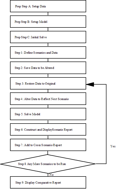
The basic structure of a comparative analysis that avoids repetitive instructions for solves and report writing is outlined in the Figure below. Note that the first three boxes represent preparatory steps that are the usual parts of a GAMS program: the initial data is set up, the model is defined and solved. The comparative model analysis begins with the box labeled "Step 1". In Step 1 names for the scenarios are introduced and the scenario data is defined. In Step 2 the base data that will be changed during the scenario runs are saved in a new parameter. We will use this parameter later to restore the data to their base levels before each new scenario run. Starting with Step 3 we enter a loop, where the looping set is the set of scenarios introduced in Step 1. As usual, the statements in the loop are executed for each scenario to be analyzed. The first statement restores the data to their base levels (Step 3). Thus we will always start with the same data. In Step 4 the data and the model is updated for the current scenario and in Step 5 the model solved. In Step 6 a report for the individual scenarios is generated. In Step 7 parameters for cross-scenario comparative reports are saved. In Step 8 we check if more scenarios are to be solved and if this is the case, we return to repeat Steps 3-8 until all scenarios are completed. Finally, we display a comparative report that presents the information saved across scenarios.
This flow chart is implemented in the file compare.gms that is given below. Note that it is based on the farm profit-maximizing example discussed in section Manual Approach above. All sets and parameters were introduced in the sections above, only the table scenprice in the implementation of Step 1 is new.
*Step 1 - Setup scenarios
Set ordr      / "Scenario Setup", "Scenario Results" /;
Set scenarios / base, beefp, beefcorn /;
Parameter savsumm(ordr,*,alli,scenarios) 'Comparative Farm Summary';
Table     scenprice(primary,scenarios)   'price changes by scenario'
                base    beefp   beefcorn
corn                               2.70
soybeans
beef                     0.70            ;

*Step 2 - Save data
Parameter savprice(primary) 'save primary commodity prices';
savprice(primary) = price(primary);


*Step 3 - Reset data to base level
loop(scenarios,
    price(primary) = savprice(primary);

*Step 4 - Change data to levels needed in scenario
    price(primary)$scenprice(primary,scenarios) = scenprice(primary,scenarios);
    display price;

*Step 5 - Solve model
   solve farm using LP maximizing netincome;

*Step 6 - Single scenario report writing
   $include farmrep.gms

*Step 7 - Cross-scenario report writing
    savsumm("Scenario Setup","price",primary,scenarios) = price(primary);
    savsumm("Scenario Results",measures,alli,scenarios) = summary(alli,measures);

*Step 8 - End of loop
    );

*Step 9 - Compute and display final results
option savsumm:2:3:1;
display savsumm;
Note that the main feature that facilitates this automatic approach is a loop statement. Loop statements are introduced and discussed in section The Loop Statement. Note further, that in Step 4 we used a conditional assignment to restrict the change of data to those primary commodities that have nonzero entries for the respective scenario in parameter scenprice. For details on conditional assignments, see section Conditional Assignments.
Adding A Scenario
Given the implementation of an automated comparative analysis above, it is easy to add a new scenario. Only two small modifications are needed: a name for the new scenario has to be added to the set scenarios and the respective data has to be added to the table scenprice. Both changes are in Step 1. The lines of the respective code are given below:
Set scenarios / base, beefp, beefcorn, new/;
Table scenprice(primary,scenarios)  'price alterations by scenario'
                base    beefp   beefcorn  new
corn                               2.70
soybeans                                  4.32
beef                     0.70                 ;
Note that we added a third alternative scenario called new, where the price of soybeans is changed to $4.32. Note further, that the remainder of the code is not changed. Once the new scenario is added to the set scenarios and the respective data is specified in the table, it will enter the loop and thus all the statements in the loop will be executed for the new scenario.
Observe that the new scenario above was similar to the other scenarios: the price for a primary commodity was modified. However, in some cases new scenarios require that other data, like resources, are changed. For example, assume that in a new scenario the landtype "cropland" is increased by 30%. Note that the available resources were defined in the parameter available(alli), where available("cropland") equals 700. To accommodate this new scenario we will add the following lines of code to Steps 1 to 4:
*Step 1 - Setup scenarios
Set scenarios / base, beefp, beefcorn, new /;
Table scenavailable(alli,scenarios)  'resource alterations by scenario'
                base    beefp   beefcorn  new
cropland                                  1.3;

*Step 2 - Save data
Parameter saveavailable (alli) 'save available resources';
saveavailable (alli) = available (alli);

*Step 3 - Reset data to base level
loop(scenarios,
    available (alli) = saveavailable (alli);

*Step 4 - Change data to levels needed in scenario
    available(alli)$scenavailable(alli,scenarios) =
       available(alli)*scenavailable(alli,scenarios);
    display price, available;
Note that in Step 1 we added a new table, scenavailable, to specify the resource alternations by scenario. Observe that the values of scenavailable will be used as multipliers in Step 4. In Step 2 we introduced the parameter saveavailable, that will play a similar role for the available resources like the parameter savprice does for the prices of the primary commodities: the base levels are saved in this parameter and we will use it to restore the values of available to their base levels before each new scenario run. This is implemented with the new assignment in Step 3. In Step 4 the data levels of the parameter available are modified as required for the current scenario using a conditional assignment. Note the similarities to the assignment for updating the values of price in Step 4 above. Steps 5 to 9 remain unchanged. Thus we achieved an automated comparative analysis with an additional scenario where another parameter is modified by adding just a few lines of code. The full code is given in the GAMS file compareother.gms.
Changing the Structure of a Model
Many studies require modifications of the structure of a model. In GAMS, context-sensitive model structures may be implemented with dollar conditions. Dollar conditions may be used to control equations as well as specific terms.
To illustrate, we will extend the profi-maximizing farm model from the previous sections to include a conditional constraint that limits the number of cattle. This constraint will be only active if a scalar that varies with the scenarios is nonzero. Consider the lines of code that follow. Note that the set animals is a subset of the set alli, the elements of the set livemanage denote various ways of managing crops and animals, and liveprod is a positive variable for livestock production.
$include farmcomp.gms
$include farmrep.gms

Scalar   cowlim   'activates cowlimit constraint' /1/;
Equation cowlimit 'conditional equation on cow limits;
cowlimit$cowlim..   sum((animals,livemanage), liveprod(animals,livemanage)) =l= 100;
Model farmcowlim /all/;

Set ordr      / "Scenario setup", "Scenario Results" /;
Set scenarios / base, cowlim /;
Parameter savprice(primary) 'save primary commodity prices';
savprice(primary) = price(primary);
Parameter cowlims(scenarios) 'cowlimit by scenario'
          / base 0, cowlim 1/;

loop(scenarios,
    cowlim = cowlims(scenarios);
    solve farmcowlim using LP maximizing netincome;
);
Note that in the loop the value of the scalar cowlim is updated before each scenario is run. Note further, that this value determines whether the new equation cowlimit will be active or not. The complete code is given in the GAMS file comparemod.gms.
Ranging analysis
Some users are interested in getting ranging output in the form of LP cost and right hand side ranging results. Unfortunately, the base version of GAMS does not yield such information. The user wishing such information has two alternatives. First, one may cause the model to be repeatedly solved under a set of values for the key parameter using the procedures discussed above, but this is cumbersome if a lot of parameters are involved. Second, one can use solver dependent features of GAMS that can be retrieved into a GAMS parameter. Please refer to the solver manuals (e.g. for GAMS/CPLEX: Sensitivity Analysis) for further information how to use them.